9. Iterative CS-based MR image reconstruction from Cartesian data

In this tutorial we will reconstruct an MR image from Cartesian under-sampled kspace measurements.

We use the toy datasets available in pysap, more specifically a 2D brain slice and the cartesian acquisition scheme. We compare zero-order image reconstruction with Compressed sensing reconstructions (analysis vs synthesis formulation) using the FISTA algorithm for the synthesis formulation and the Condat-Vu algorithm for the analysis formulation.Sparsity will be promoted in the wavelet domain, using either Symmlet-8 (analysis and synthesis) or undecimated bi-orthogonal wavelets (analysis only).

We remind that the synthesis formulation reads (minimization in the sparsifying domain):

\widehat{z} = \text{arg}\,\min_{z\in C^n_\Psi} \frac{1}{2} \|y - \Omega F \Psi^*z \|_2^2 + \lambda \|z\|_1

(1)

and the image solution is given by $\widehat{x} = \Psi^*\widehat{z}$ . For an orthonormal wavelet transform, we have $n_\Psi=n$ while for a frame we may have $n_\Psi > n$ .

while the analysis formulation consists in minimizing the following cost function (min. in the image domain):

\widehat{x} = \text{arg}\,\min_{x\in C^n} \frac{1}{2} \|y - \Omega F x\|_2^2 + \lambda \|\Psi x\|_1 \,.

(2)

Author: Chaithya G R & Philippe Ciuciu
Date: 01/06/2021
Update: 04/02/2025
Target: ATSI MSc students, Paris-Saclay University

#DISPLAY BRAIN PHANTOM
%matplotlib inline

import numpy as np
from mri.operators.utils import convert_mask_to_locations
from mri.reconstructors import SingleChannelReconstructor
from mri.operators import FFT, WaveletN, WaveletUD2
import os.path as op
import os
import math ; import cmath
import matplotlib.pyplot as plt
import sys
from modopt.math.metrics import ssim
from modopt.opt.proximity import SparseThreshold
from modopt.opt.linear import Identity

from skimage import data, io, filters

import pywt as pw
import matplotlib.pyplot as plt

import brainweb_dl as bwdl

plt.rcParams["image.origin"]="lower"
plt.rcParams["image.cmap"]='Greys_r'

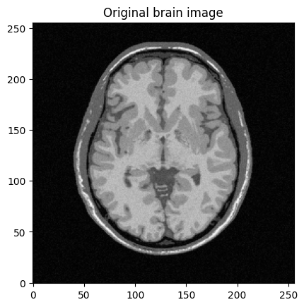
mri_img = bwdl.get_mri(4, "T1")[70, ...].astype(np.float32)
#mri_img = bwdl.get_mri(4, "T2")[120, ...].astype(np.float32)
print(mri_img.shape)
img_size = mri_img.shape[0]
plt.figure()
plt.imshow(abs(mri_img))
plt.title("Original brain image")
plt.show()

(256, 256)

#image = get_sample_data('2d-mri')
# Obtain K-Space Cartesian Mask
#mask = get_sample_data("cartesian-mri-mask")
image = mri_img 
from mrinufft.trajectories.tools import get_random_loc_1d

phase_encoding_locs = get_random_loc_1d(image.shape[0], accel=8, center_prop=0.1, pdf='gaussian')
print(phase_encoding_locs, min(phase_encoding_locs), max(phase_encoding_locs))
phase_encoding_locs = ((phase_encoding_locs +0.5) * image.shape[0]).astype(int)
mask = np.zeros(image.shape, dtype=bool)
mask[phase_encoding_locs] = 1

[ 0.          0.00390625 -0.00390625  0.0078125  -0.0078125   0.01171875
 -0.01171875  0.015625   -0.015625    0.01953125 -0.01953125  0.0234375
 -0.0234375   0.02734375 -0.02734375  0.03125    -0.03125     0.03515625
 -0.03515625  0.0390625  -0.0390625   0.04296875 -0.04296875  0.078125
 -0.046875    0.0859375  -0.05078125  0.09765625 -0.06640625  0.10546875
 -0.1015625   0.1484375  -0.140625    0.16796875 -0.1484375   0.1796875
 -0.16015625  0.1875     -0.16796875  0.203125   -0.171875    0.21484375
 -0.17578125  0.2265625  -0.20703125  0.28515625 -0.25390625  0.34765625
 -0.26171875  0.3828125  -0.265625   -0.27734375 -0.33984375] -0.33984375 0.3828125

plt.subplot(1, 2, 1)
plt.imshow(np.abs(image), cmap='gray')
plt.title("MRI Data")
plt.subplot(1, 2, 2)
plt.imshow(mask, cmap='gray')
plt.title("K-space Sampling Mask")
plt.show()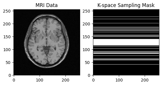

Generate the kspace¶

From the 2D brain slice and the acquisition mask, we retrospectively undersample the k-space using a cartesian acquisition mask. We then reconstruct the zero order solution as a baseline

Get the locations of the kspace samples

# Get the locations of the kspace samples
kspace_loc = convert_mask_to_locations(mask)
# Generate the subsampled kspace
fourier_op = FFT(samples=kspace_loc, shape=image.shape)
kspace_data = fourier_op.op(image)

Zero order solution

zero_soln = fourier_op.adj_op(kspace_data)
base_ssim = ssim(zero_soln, image)
plt.imshow(np.abs(zero_soln), cmap='gray')
plt.title('Zero Order Solution : SSIM = ' + str(np.around(base_ssim, 3)))
plt.show()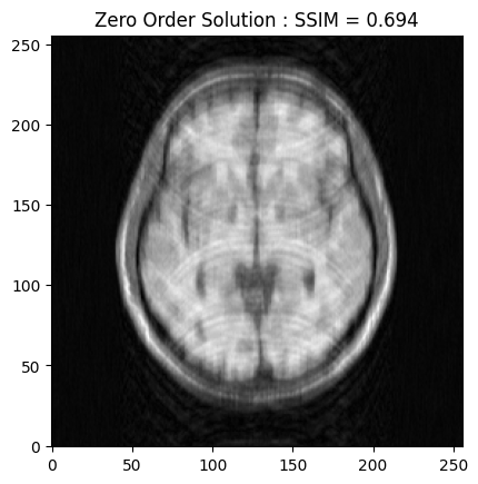

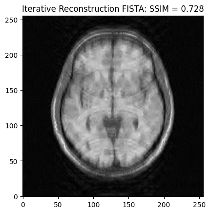
Synthesis formulation: FISTA vs POGM optimization¶

We now want to refine the zero-order solution using compressed sensing reconstruction. Here we adopt the synthesis formulation based on the FISTA algorithm. The cost function is set to Proximity Cost + Gradient Cost

# Setup the operators
linear_op = WaveletN(wavelet_name="sym8", nb_scales=4)
regularizer_op = SparseThreshold(Identity(), 0.1, thresh_type="soft")
# Setup Reconstructor
reconstructor = SingleChannelReconstructor(
    fourier_op=fourier_op,
    linear_op=linear_op,
    regularizer_op=regularizer_op,
    gradient_formulation='synthesis',
    verbose=1,
)

Lipschitz constant is 1.0999999782973517

WARNING: Making input data immutable.

image_rec, costs, metrics = reconstructor.reconstruct(
    kspace_data=kspace_data,
    optimization_alg='fista',
    num_iterations=200,
)
recon_ssim = ssim(image_rec, image)
plt.imshow(np.abs(image_rec), cmap='gray')
plt.title('Iterative Reconstruction FISTA: SSIM = ' + str(np.around(recon_ssim, 3)))
plt.show()

 - mu:  0.1
 - lipschitz constant:  1.0999999782973517
 - data:  (256, 256)
 - wavelet:  <mri.operators.linear.wavelet.WaveletN object at 0x794b8fe7b100> - 4
 - max iterations:  200
 - image variable shape:  (256, 256)
 - alpha variable shape:  (81225,)
----------------------------------------
Starting optimization...

 - final iteration number:  200
 - final log10 cost value:  6.0
 - converged:  False
Done.
Execution time:  5.970125935000397  seconds
----------------------------------------

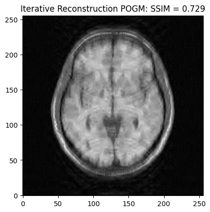
POGM optimization¶

image_rec2, costs, metrics = reconstructor.reconstruct(
    kspace_data=kspace_data,
    optimization_alg='pogm',
    num_iterations=200,
)
recon2_ssim = ssim(image_rec2, image)
plt.imshow(np.abs(image_rec2), cmap='gray')
plt.title('Iterative Reconstruction POGM: SSIM = ' + str(np.around(recon2_ssim, 3)))
plt.show()

 - mu:  0.1
 - lipschitz constant:  1.0999999782973517
 - data:  (256, 256)
 - wavelet:  <mri.operators.linear.wavelet.WaveletN object at 0x794b8fe7b100> - 4
 - max iterations:  200
 - image variable shape:  (1, 256, 256)
----------------------------------------
Starting optimization...

 - final iteration number:  200
 - final log10 cost value:  6.0
 - converged:  False
Done.
Execution time:  6.327495501001977  seconds
----------------------------------------

Analysis formulation: Condat-Vu reconstruction¶

linear_op = WaveletUD2(
    wavelet_id=24,
    nb_scale=4,
)
regularizer_op = SparseThreshold(Identity(), 0.1, thresh_type="soft")

reconstructor = SingleChannelReconstructor(
    fourier_op=fourier_op,
    linear_op=linear_op,
    regularizer_op=regularizer_op,
    gradient_formulation='analysis',
    verbose=1,
)

Lipschitz constant is 1.0999999972637438

WARNING: Making input data immutable.

image_rec3, costs, metrics = reconstructor.reconstruct(
    kspace_data=kspace_data,
    optimization_alg='condatvu',
    num_iterations=200,
)
recon3_ssim = ssim(image_rec3, image)
plt.imshow(np.abs(image_rec3), cmap='gray')
plt.title('Iterative Reconstruction Condat-Vu: SSIM = ' + str(np.around(recon3_ssim, 3)))
plt.show()

 - mu:  0.1
 - lipschitz constant:  1.0999999972637438
 - tau:  0.9374654938140249
 - sigma:  0.5
 - rho:  1.0
 - std:  None
 - 1/tau - sigma||L||^2 >= beta/2:  True
 - data:  (256, 256)
 - wavelet:  <mri.operators.linear.wavelet.WaveletUD2 object at 0x794b8fd89420> - 4
 - max iterations:  200
 - number of reweights:  0
 - primal variable shape:  (256, 256)
 - dual variable shape:  (655360,)
----------------------------------------
Starting optimization...

WARNING: <class 'mri.operators.linear.wavelet.WaveletUD2'> does not inherit an operator parent.

 - final iteration number:  200
 - final cost value:  1000000.0
 - converged:  False
Done.
Execution time:  99.8788210040002  seconds
----------------------------------------