1. Basic deterministic under-sampling - MRI acquisition and Reconstruction

In this first notebook, we start with simple deterministic under-sampling using either a low-frequency or a high-frequency mask. Hence we want to generate a sampling mask $\Omega\in\{0,1\}^N$ such that $y = F_{\Omega} x$ where $x\in R^{N}$ is the original image. The data $y$ is then corrupted by additive noise $b$ :

y = F_{\Omega} x + b

(1)

where $b$ is a complex-valued circular Gaussian noise of variance $\sigma^2$ and $F_{\Omega} = \Omega F$ in this Cartesian setting (i.e. sampling on the grid). We consider:

a low-frequency Cartesian mask $\Omega$ is defined by the central lines of k-space.
a low-frequency Cartesian mask $\Omega$ is defined by a square box in k-space centered at $(k_x,k_y)=(0,0)$ .
a high-frequency Cartesian mask $\Omega$ is defined as the complementary set of the lines defined in to 1)
a high-frequency Cartesian mask $\Omega$ is defined as the complementary set of the box defined in 2)

Based on these masks we generate the corresponding measured data from a reference MR image and finally perform Cartesian image reconstruction $\widehat{x}$ from the under-sampled data $y$ as follows:

\widehat{x} = \tilde{F}^* y

(2)

where $F^*$ is the zero-filled inverse Fourier transform (ifft).

Author: Philippe Ciuciu (philippe.ciuciu@cea.fr)
Date: 02/03/2025
Target: IEEE EMBS-SPS Summer School on Novel acquisition and image reconstruction strategies in accelerated Magnetic Resonance Imaging

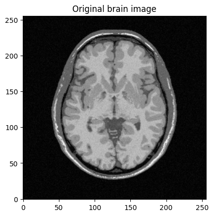
#DISPLAY BRAIN PHANTOM
%matplotlib inline
import sys
import os.path as op
import os
import math
import cmath

import numpy as np

import matplotlib.pyplot as plt

from skimage import data, io
import brainweb_dl as bwdl

plt.rcParams["image.origin"]="lower"
plt.rcParams["image.cmap"]='Greys_r'

mri_img = bwdl.get_mri(4, "T1")[70, ...].astype(np.float32)
#mri_img = bwdl.get_mri(4, "T2")[120, ...].astype(np.float32)
print(mri_img.shape)
img_size = mri_img.shape[0]
plt.figure()
plt.imshow(abs(mri_img))
#plt.imshow(abs(mri_2D),origin="lower")
#plt.imshow(abs(mri_2D),origin="upper")
plt.title("Original brain image")
plt.show()

(256, 256)

To get started, the objective is to build a low-frequency sampling mask that consists of the central k-space lines
Fourier transform the reference MR image to compute k-space data, add zero-mean Gaussian complex-valued noise
Mask the data using the above defined mask
Next, perform zero-filled MR image reconstruction from masked k-space data
Study the impact of the number of lines in the mask on the final image quality

# Generate trivial Cartesian sampling masks
#img_size = 512

mask="low_res"
factor_ctr = 4

#Objective: construct a k-space mask that consists of the central lines
# 0 entries: points not sampled, 1 entries: points to be sampled
# Initialize k-space with 0 everywhere and then place the "1" appropriately
kspace_masklines = np.zeros((img_size,img_size), dtype="float64")

low_res_size = img_size // factor_ctr + 1
idx_vec = np.linspace(img_size // 2 - low_res_size // 2, img_size // 2 + low_res_size // 2, low_res_size)
idx_vec_ =  idx_vec.astype("int")
#print(idx_vec_)

#Use fancy indexing to select low frequency lines only
kspace_masklines[idx_vec_, ] = 1


if 0:
    plt.figure()
    plt.imshow(kspace_masklines, cmap='Greys_r')
    plt.title("Sampling mask")
    plt.show()

norm = "ortho"
#norm = None

def fft(x):
    return np.fft.fft2(x, norm=norm)

def ifft(x):
    return np.fft.ifft2(x, norm=norm)

# Generate the kspace data: first Fourier transform the image
kspace_data = np.fft.fftshift(fft(mri_img))
#add Gaussian complex-valued random noise
signoise = 10
#kspace_data += np.random.randn(*mri_img.shape) * signoise * (1+1j)
# Simulate independent noise realization on the real & imag parts
kspace_data += (np.random.randn(*mri_img.shape) + 1j*np.random.randn(*mri_img.shape)) * signoise
# Mask data to perform subsampling
kspace_data *= kspace_masklines

# Zero order solution
image_rec0 = ifft(np.fft.ifftshift(kspace_data))            # get back to the convention

fig, axs = plt.subplots(2, 2, figsize=(10, 10))
axs[0, 0].imshow(mri_img)
axs[0, 0].set_title("True image")
axs[0, 1].imshow(kspace_masklines)
axs[0, 1].set_title("Low frequency sampling mask")
axs[1, 0].imshow(np.abs(kspace_data), vmax=0.01*np.abs(kspace_data).max())
axs[1, 0].set_title("k-space noisy data")
axs[1, 1].imshow(np.abs(image_rec0))
axs[1, 1].set_title("Zero-order recon")
plt.show()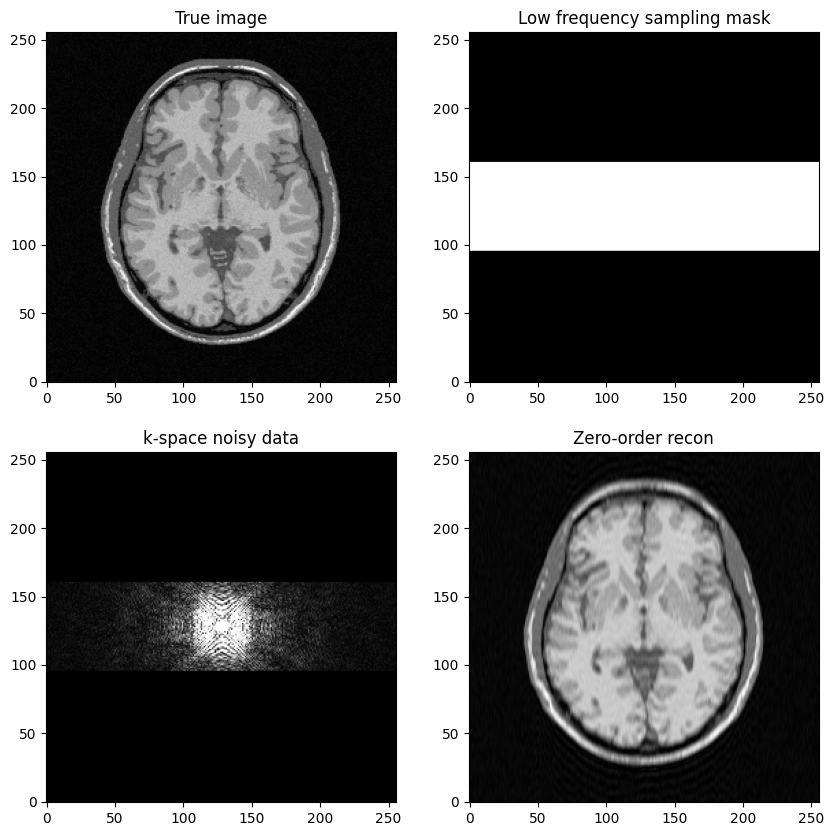

Question: based on the previous example, try to construct a low-freqency sampling mask defined by a square box centered around $(k_x, k_y) = (0,0)$ .
Then, replicate the same steps:
1. Generate noisy masked data
2. Perform zero-filled MR image reconstruction
3. Visualize results and study the impact of both the noise level and the mask size

#Objective: construct a k-space mask consisting of a central box
# Initialize k-space with 0 everywhere and then place the "1" appropriately
kspace_maskbox = np.zeros((img_size,img_size), dtype="float64")
# use fancy indexing along rows
kspace_maskbox[idx_vec_, ] = 1

list_img_size = np.arange(0., img_size).tolist()
filtered_center = [x for x in list_img_size if x not in idx_vec_]
array_idx_center = np.array(filtered_center)
array_idx_center_ = array_idx_center.astype("int")
# use fancy indexing along cols
kspace_maskbox[:, array_idx_center_] = 0

# Generate the kspace data: first Fourier transform the image
kspace_data = np.fft.fftshift(fft(mri_img))
#add Gaussian complex-valued random noise
signoise = 10
# Simulate independent noise realization on the real & imag parts
kspace_data += (np.random.randn(*mri_img.shape) + 1j * np.random.randn(*mri_img.shape)) * signoise
# Mask data to perform subsampling
kspace_data *= kspace_maskbox

fig, axs = plt.subplots(2, 2, figsize=(10, 10))
axs[0, 0].imshow(mri_img)
axs[0, 0].set_title("True image")
axs[0, 1].imshow(kspace_maskbox)
axs[0, 1].set_title("Low frequency sampling mask")
axs[1, 0].imshow(np.abs(kspace_data),  vmax=0.01*np.abs(kspace_data).max())
axs[1, 0].set_title("k-space noisy data")
axs[1, 1].imshow(np.abs(image_rec0))
axs[1, 1].set_title("Zero-order recon")
plt.show()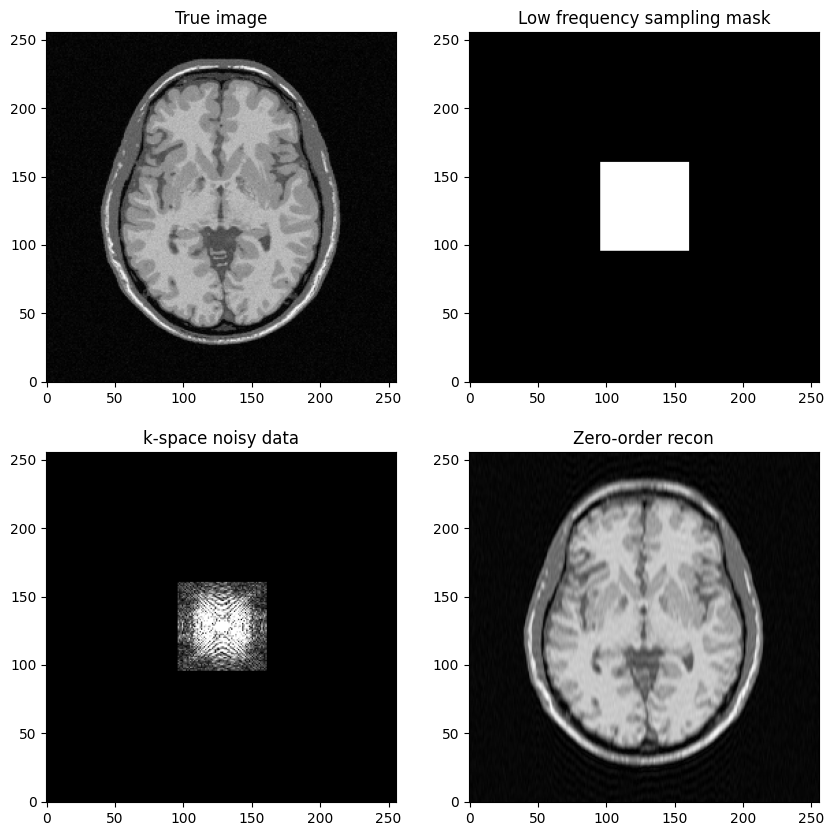

Next question: Construct a k-space sampling mask that consists of the high-frequency lines, just discard the central lines
Study the impact of the number of lines removed

# 0 entries: points not sampled, 1 entries: points to be sampled
# Initialize k-space with "1" everywhere and then place the "0" appropriately

kspace_masklines = np.ones((img_size,img_size), dtype="float64")
low_res_size = img_size // factor_ctr + 1
idx_vec_upper = np.linspace(img_size // 2 - low_res_size // 2, img_size // 2 + low_res_size // 2, low_res_size)
idx_vec_upper_ =  idx_vec.astype("int")

# set central k-space lines to 0: use fancy indexing along rows
kspace_masklines[idx_vec_upper_, ] = 0

# Generate the kspace data: first Fourier transform the image
kspace_data = np.fft.fftshift(fft(mri_img))
#add Gaussian complex-valued random noise
signoise = 10
#kspace_data += np.random.randn(*mri_img.shape) * signoise * (1+1j)
# Simulate independent noise realization on the real & imag parts
kspace_data += (np.random.randn(*mri_img.shape) + 1j * np.random.randn(*mri_img.shape)) * signoise
# Mask data to perform subsampling
kspace_data *= kspace_masklines

# Zero order solution
image_rec0 = ifft(np.fft.ifftshift(kspace_data))            # get back to the convention

fig, axs = plt.subplots(2, 2, figsize=(10, 10))
axs[0, 0].imshow(mri_img)
axs[0, 0].set_title("True image")
axs[0, 1].imshow(kspace_masklines)
axs[0, 1].set_title("High frequency sampling mask")
axs[1, 0].imshow(np.abs(kspace_data),  vmax=0.01*np.abs(kspace_data).max())
#axs[1].imshow(np.abs(np.fft.ifftshift(kspace_data)), cmap='Greys_r')
axs[1, 0].set_title("k-space noisy data")
axs[1, 1].imshow(np.abs(image_rec0))
axs[1, 1].set_title("Zero-order recon")
plt.show()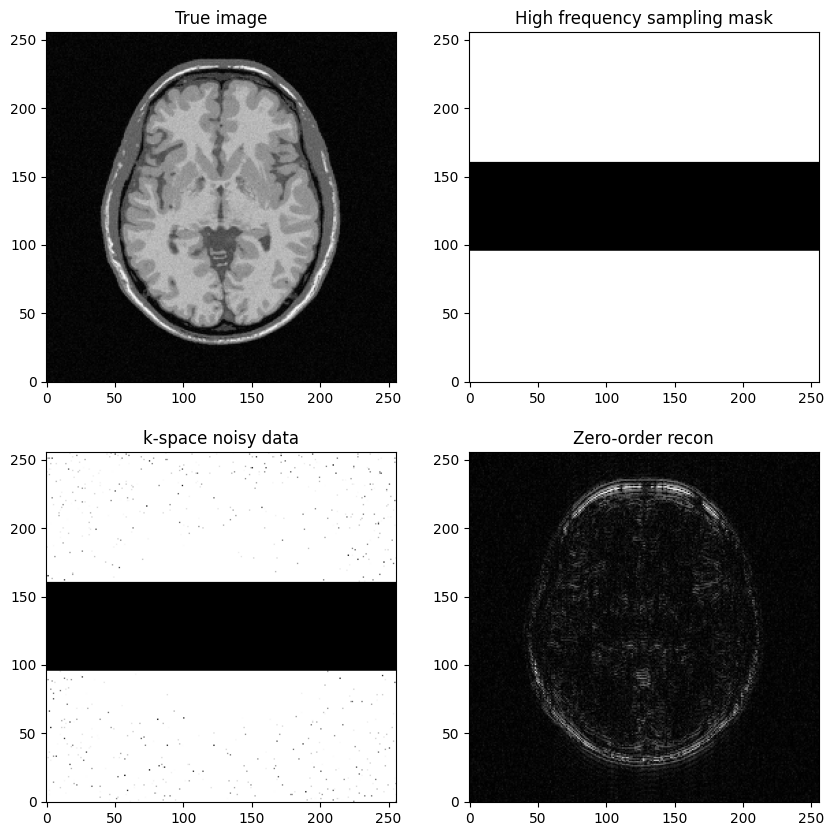

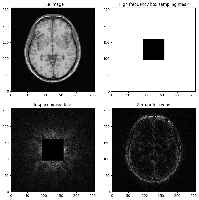
Question: Based on the previous example, try to construct a k-space mask that consists of the removing the central box centered in $(𝑘_𝑥,𝑘_𝑦)=(0,0)$ .

Then, replicate the same steps:
1. Generate noisy masked data
2. Perform zero-filled MR image recon
3. Visualize results and study the impact of both the noise level and the mask size

# 0 entries: points not sampled, 1 entries: points to be sampled
# Initialize k-space with "1" everywhere and then place the "0" appropriately
kspace_maskbox = np.ones((img_size,img_size), dtype="float64")
# use fancy indexing along rows
kspace_maskbox[idx_vec_, ] = 0

list_img_size = np.arange(0., img_size).tolist()
filtered_center = [x for x in list_img_size if x not in idx_vec_]
array_idx_center = np.array(filtered_center)
array_idx_center_ = array_idx_center.astype("int")
# use fancy indexing along cols
kspace_maskbox[:, array_idx_center_] = 1

# Generate the kspace data: first Fourier transform the image
kspace_data = np.fft.fftshift(fft(mri_img))
#add Gaussian complex-valued random noise
signoise = 10
#kspace_data += np.random.randn(*mri_img.shape) * signoise * (1+1j)
# Simulate independent noise realization on the real & imag parts
kspace_data += (np.random.randn(*mri_img.shape) + 1j*np.random.randn(*mri_img.shape)) * signoise
# Mask data to perform subsampling
kspace_data *= kspace_maskbox

# Zero order solution
image_rec0 = ifft(np.fft.ifftshift(kspace_data))

fig, axs = plt.subplots(2, 2, figsize=(10, 10) )
axs[0,0].imshow(mri_img, cmap='Greys_r')
axs[0,0].set_title("True image")
axs[0,1].imshow(kspace_maskbox, cmap='Greys_r')
axs[0,1].set_title("High frequency box sampling mask")
axs[1,0].imshow(np.abs(kspace_data),  cmap='gray', vmax=1*np.abs(kspace_data).max())
#axs[1].imshow(np.abs(np.fft.ifftshift(kspace_data)), cmap='Greys_r')
axs[1,0].set_title("k-space noisy data")
axs[1,1].imshow(np.abs(image_rec0), cmap='Greys_r')
axs[1,1].set_title("Zero-order recon")
plt.show()