Note
Go to the end to download the full example code.
Creating motion artifacts on an anatomical EPI with SNAKE-fMRI#
This examples walks through the elementary components of SNAKE and demonstrates how to add motion artifacts to the simulation.
# Imports
import numpy as np
import matplotlib.pyplot as plt

from snake.core.phantom import Phantom
from snake.core.sampling import EPI3dAcquisitionSampler
from snake.core.simulation import GreConfig, SimConfig, default_hardware
Setting up the base simulation Config. This configuration holds all key parameters for the simulation, describing the scanner parameters.
sim_conf = SimConfig(
    max_sim_time=6,
    seq=GreConfig(TR=50, TE=30, FA=3),
    hardware=default_hardware,
)
sim_conf.hardware.n_coils = 8
sim_conf.fov.res_mm = (3, 3, 3)
sim_conf
Creating the base Phantom#
The simulation acquires the data describe in a phantom. A phantom consists of fuzzy segmentation of head tissue, and their MR intrinsic parameters (density, T1, T2, T2*, magnetic susceptibilities)
Here we use Brainweb reference mask and values for convenience.
phantom = Phantom.from_brainweb(
    sub_id=4, sim_conf=sim_conf, output_res=1, tissue_file="tissue_7T"
)

# Here are the tissue availables and their parameters
phantom.affine
No matrix size found in the header. The header is probably missing.

array([[1., 0., 0., 0.],
       [0., 1., 0., 0.],
       [0., 0., 1., 0.],
       [0., 0., 0., 1.]], dtype=float32)
Adding motion to the Phantom#
The motion is added to the phantom by applying a transformation to the simulation’s FOV configuration (as if the phantom was moving in the scanner).
from snake.core.handlers import RandomMotionImageHandler

motion = RandomMotionImageHandler(
    ts_std_mms=[1, 1, 1],
    rs_std_degs=[0.1, 0.1, 0.1],
)

motion2 = RandomMotionImageHandler(
    ts_std_mms=[3, 3, 3],
    rs_std_degs=[0.5, 0.5, 0.5],
)
Setting up Acquisition Pattern and Initializing Result file.#
# The next piece of simulation is the acquisition trajectory.
# Here nothing fancy, we are using a EPI (fully sampled), that samples a 3D
# k-space (this akin to the 3D EPI sequence of XXXX)

sampler = EPI3dAcquisitionSampler(accelz=1, acsz=0.1, orderz="top-down")
Acquisition with Cartesian Engine#
We acquire the three setup separately.
from snake.core.engine import EPIAcquisitionEngine

engine = EPIAcquisitionEngine(model="simple")

engine(
    "example_nomotion.mrd",
    sampler=sampler,
    phantom=phantom,
    handlers=[],
    sim_conf=sim_conf,
    worker_chunk_size=16,
    n_workers=4,
)

engine(
    "example_motion.mrd",
    sampler=sampler,
    phantom=phantom,
    handlers=[motion],
    sim_conf=sim_conf,
    worker_chunk_size=16,
    n_workers=4,
)

engine(
    "example_motion2.mrd",
    sampler=sampler,
    phantom=phantom,
    handlers=[motion2],
    sim_conf=sim_conf,
    worker_chunk_size=16,
    n_workers=4,
)
Existing example_nomotion.mrd it will be overwritten
[Errno 2] No such file or directory: 'example_nomotion.mrd'

  0%|          | 0/120 [00:00<?, ?it/s]
  1%|          | 1/120 [00:00<00:49,  2.38it/s]
  2%|▏         | 2/120 [00:00<00:27,  4.22it/s]
  2%|▎         | 3/120 [00:00<00:20,  5.61it/s]
  3%|▎         | 4/120 [00:00<00:17,  6.62it/s]
  4%|▍         | 5/120 [00:00<00:15,  7.37it/s]
  5%|▌         | 6/120 [00:00<00:14,  7.90it/s]
  6%|▌         | 7/120 [00:01<00:13,  8.31it/s]
  7%|▋         | 8/120 [00:01<00:13,  8.56it/s]
  8%|▊         | 9/120 [00:01<00:12,  8.70it/s]
  8%|▊         | 10/120 [00:01<00:12,  8.86it/s]
  9%|▉         | 11/120 [00:01<00:12,  8.89it/s]
 10%|█         | 12/120 [00:01<00:12,  8.85it/s]
 11%|█         | 13/120 [00:01<00:12,  8.77it/s]
 12%|█▏        | 14/120 [00:01<00:12,  8.78it/s]
 12%|█▎        | 15/120 [00:01<00:11,  8.91it/s]
 13%|█▎        | 16/120 [00:02<00:11,  9.02it/s]
 14%|█▍        | 17/120 [00:02<00:11,  9.05it/s]
 15%|█▌        | 18/120 [00:02<00:11,  9.09it/s]
 16%|█▌        | 19/120 [00:02<00:11,  9.08it/s]
 17%|█▋        | 20/120 [00:02<00:10,  9.12it/s]
 18%|█▊        | 21/120 [00:02<00:10,  9.14it/s]
 18%|█▊        | 22/120 [00:02<00:10,  9.07it/s]
 19%|█▉        | 23/120 [00:02<00:10,  9.11it/s]
 20%|██        | 24/120 [00:02<00:10,  9.12it/s]
 21%|██        | 25/120 [00:03<00:10,  9.14it/s]
 22%|██▏       | 26/120 [00:03<00:10,  9.18it/s]
 22%|██▎       | 27/120 [00:03<00:10,  9.14it/s]
 23%|██▎       | 28/120 [00:03<00:10,  9.14it/s]
 24%|██▍       | 29/120 [00:03<00:09,  9.13it/s]
 25%|██▌       | 30/120 [00:03<00:09,  9.14it/s]
 26%|██▌       | 31/120 [00:03<00:09,  9.12it/s]
 27%|██▋       | 32/120 [00:03<00:09,  9.10it/s]
 28%|██▊       | 33/120 [00:03<00:09,  8.99it/s]
 28%|██▊       | 34/120 [00:04<00:09,  9.00it/s]
 29%|██▉       | 35/120 [00:04<00:09,  9.03it/s]
 30%|███       | 36/120 [00:04<00:09,  9.05it/s]
 31%|███       | 37/120 [00:04<00:09,  8.98it/s]
 32%|███▏      | 38/120 [00:04<00:09,  9.01it/s]
 32%|███▎      | 39/120 [00:04<00:08,  9.02it/s]
 33%|███▎      | 40/120 [00:04<00:08,  9.06it/s]
 34%|███▍      | 41/120 [00:04<00:08,  9.09it/s]
 35%|███▌      | 42/120 [00:04<00:08,  9.11it/s]
 36%|███▌      | 43/120 [00:05<00:08,  9.14it/s]
 37%|███▋      | 44/120 [00:05<00:08,  9.18it/s]
 38%|███▊      | 45/120 [00:05<00:08,  9.17it/s]
 38%|███▊      | 46/120 [00:05<00:08,  9.20it/s]
 39%|███▉      | 47/120 [00:05<00:08,  9.12it/s]
 40%|████      | 48/120 [00:05<00:07,  9.19it/s]
 41%|████      | 49/120 [00:05<00:07,  9.23it/s]
 42%|████▏     | 50/120 [00:05<00:07,  9.23it/s]
 42%|████▎     | 51/120 [00:05<00:07,  9.20it/s]
 43%|████▎     | 52/120 [00:06<00:07,  9.18it/s]
 44%|████▍     | 53/120 [00:06<00:07,  9.12it/s]
 45%|████▌     | 54/120 [00:06<00:07,  9.15it/s]
 46%|████▌     | 55/120 [00:06<00:07,  9.13it/s]
 47%|████▋     | 56/120 [00:06<00:07,  9.14it/s]
 48%|████▊     | 57/120 [00:06<00:06,  9.12it/s]
 48%|████▊     | 58/120 [00:06<00:06,  9.12it/s]
 49%|████▉     | 59/120 [00:06<00:06,  9.09it/s]
 50%|█████     | 60/120 [00:06<00:06,  9.09it/s]
 51%|█████     | 61/120 [00:07<00:06,  9.11it/s]
 52%|█████▏    | 62/120 [00:07<00:06,  9.12it/s]
 52%|█████▎    | 63/120 [00:07<00:06,  9.09it/s]
 53%|█████▎    | 64/120 [00:07<00:06,  9.10it/s]
 54%|█████▍    | 65/120 [00:07<00:06,  9.11it/s]
 55%|█████▌    | 66/120 [00:07<00:05,  9.13it/s]
 56%|█████▌    | 67/120 [00:07<00:05,  9.12it/s]
 57%|█████▋    | 68/120 [00:07<00:05,  9.13it/s]
 57%|█████▊    | 69/120 [00:07<00:05,  9.15it/s]
 58%|█████▊    | 70/120 [00:07<00:05,  9.15it/s]
 59%|█████▉    | 71/120 [00:08<00:05,  9.20it/s]
 60%|██████    | 72/120 [00:08<00:05,  9.23it/s]
 61%|██████    | 73/120 [00:08<00:05,  9.23it/s]
 62%|██████▏   | 74/120 [00:08<00:04,  9.24it/s]
 62%|██████▎   | 75/120 [00:08<00:04,  9.22it/s]
 63%|██████▎   | 76/120 [00:08<00:04,  9.26it/s]
 64%|██████▍   | 77/120 [00:08<00:04,  9.27it/s]
 65%|██████▌   | 78/120 [00:08<00:04,  9.27it/s]
 66%|██████▌   | 79/120 [00:08<00:04,  9.17it/s]
 67%|██████▋   | 80/120 [00:09<00:04,  9.15it/s]
 68%|██████▊   | 81/120 [00:09<00:04,  9.18it/s]
 68%|██████▊   | 82/120 [00:09<00:04,  9.16it/s]
 69%|██████▉   | 83/120 [00:09<00:04,  9.18it/s]
 70%|███████   | 84/120 [00:09<00:03,  9.15it/s]
 71%|███████   | 85/120 [00:09<00:03,  9.16it/s]
 72%|███████▏  | 86/120 [00:09<00:03,  9.15it/s]
 72%|███████▎  | 87/120 [00:09<00:03,  9.14it/s]
 73%|███████▎  | 88/120 [00:09<00:03,  9.06it/s]
 74%|███████▍  | 89/120 [00:10<00:03,  9.07it/s]
 75%|███████▌  | 90/120 [00:10<00:03,  9.11it/s]
 76%|███████▌  | 91/120 [00:10<00:03,  9.11it/s]
 77%|███████▋  | 92/120 [00:10<00:03,  9.13it/s]
 78%|███████▊  | 93/120 [00:10<00:02,  9.14it/s]
 78%|███████▊  | 94/120 [00:10<00:02,  9.15it/s]
 79%|███████▉  | 95/120 [00:10<00:02,  9.19it/s]
 80%|████████  | 96/120 [00:10<00:02,  9.22it/s]
 81%|████████  | 97/120 [00:10<00:02,  9.21it/s]
 82%|████████▏ | 98/120 [00:11<00:02,  9.23it/s]
 82%|████████▎ | 99/120 [00:11<00:02,  9.18it/s]
 83%|████████▎ | 100/120 [00:11<00:02,  9.14it/s]
 84%|████████▍ | 101/120 [00:11<00:02,  9.15it/s]
 85%|████████▌ | 102/120 [00:11<00:01,  9.15it/s]
 86%|████████▌ | 103/120 [00:11<00:01,  9.16it/s]
 87%|████████▋ | 104/120 [00:11<00:01,  9.11it/s]
 88%|████████▊ | 105/120 [00:11<00:01,  9.09it/s]
 88%|████████▊ | 106/120 [00:11<00:01,  9.08it/s]
 89%|████████▉ | 107/120 [00:12<00:01,  9.05it/s]
 90%|█████████ | 108/120 [00:12<00:01,  9.07it/s]
 91%|█████████ | 109/120 [00:12<00:01,  9.07it/s]
 92%|█████████▏| 110/120 [00:12<00:01,  9.05it/s]
 92%|█████████▎| 111/120 [00:12<00:00,  9.05it/s]
 93%|█████████▎| 112/120 [00:12<00:00,  9.07it/s]
 94%|█████████▍| 113/120 [00:12<00:00,  9.06it/s]
 95%|█████████▌| 114/120 [00:12<00:00,  8.87it/s]
 96%|█████████▌| 115/120 [00:12<00:00,  8.90it/s]
 97%|█████████▋| 116/120 [00:13<00:00,  8.92it/s]
 98%|█████████▊| 117/120 [00:13<00:00,  8.97it/s]
 98%|█████████▊| 118/120 [00:13<00:00,  9.02it/s]
 99%|█████████▉| 119/120 [00:13<00:00,  9.06it/s]
100%|██████████| 120/120 [00:13<00:00,  9.10it/s]
100%|██████████| 120/120 [00:13<00:00,  8.91it/s]
No coil_cov found in the dataset.

  0%|          | 0/120 [00:00<?, ?it/s]
 13%|█▎        | 16/120 [00:06<00:41,  2.48it/s]
 27%|██▋       | 32/120 [00:07<00:16,  5.21it/s]
 40%|████      | 48/120 [00:07<00:08,  8.54it/s]
 53%|█████▎    | 64/120 [00:08<00:04, 12.34it/s]
 67%|██████▋   | 80/120 [00:08<00:02, 16.50it/s]
 80%|████████  | 96/120 [00:08<00:01, 20.93it/s]
 93%|█████████▎| 112/120 [00:09<00:00, 24.93it/s]
128it [00:09, 28.60it/s]
128it [00:09, 12.89it/s]
Existing example_motion.mrd it will be overwritten
[Errno 2] No such file or directory: 'example_motion.mrd'

  0%|          | 0/120 [00:00<?, ?it/s]
  1%|          | 1/120 [00:00<00:13,  8.97it/s]
  2%|▏         | 2/120 [00:00<00:13,  8.95it/s]
  2%|▎         | 3/120 [00:00<00:12,  9.04it/s]
  3%|▎         | 4/120 [00:00<00:12,  9.09it/s]
  4%|▍         | 5/120 [00:00<00:12,  9.10it/s]
  5%|▌         | 6/120 [00:00<00:12,  9.13it/s]
  6%|▌         | 7/120 [00:00<00:12,  9.15it/s]
  7%|▋         | 8/120 [00:00<00:12,  9.11it/s]
  8%|▊         | 9/120 [00:00<00:12,  9.14it/s]
  8%|▊         | 10/120 [00:01<00:12,  9.07it/s]
  9%|▉         | 11/120 [00:01<00:11,  9.10it/s]
 10%|█         | 12/120 [00:01<00:11,  9.07it/s]
 11%|█         | 13/120 [00:01<00:11,  9.06it/s]
 12%|█▏        | 14/120 [00:01<00:11,  9.06it/s]
 12%|█▎        | 15/120 [00:01<00:11,  9.07it/s]
 13%|█▎        | 16/120 [00:01<00:11,  9.09it/s]
 14%|█▍        | 17/120 [00:01<00:11,  9.09it/s]
 15%|█▌        | 18/120 [00:01<00:11,  9.09it/s]
 16%|█▌        | 19/120 [00:02<00:11,  9.11it/s]
 17%|█▋        | 20/120 [00:02<00:10,  9.11it/s]
 18%|█▊        | 21/120 [00:02<00:10,  9.12it/s]
 18%|█▊        | 22/120 [00:02<00:10,  9.10it/s]
 19%|█▉        | 23/120 [00:02<00:10,  9.09it/s]
 20%|██        | 24/120 [00:02<00:10,  9.10it/s]
 21%|██        | 25/120 [00:02<00:10,  9.10it/s]
 22%|██▏       | 26/120 [00:02<00:10,  9.10it/s]
 22%|██▎       | 27/120 [00:02<00:10,  9.09it/s]
 23%|██▎       | 28/120 [00:03<00:10,  9.06it/s]
 24%|██▍       | 29/120 [00:03<00:09,  9.13it/s]
 25%|██▌       | 30/120 [00:03<00:09,  9.14it/s]
 26%|██▌       | 31/120 [00:03<00:09,  9.17it/s]
 27%|██▋       | 32/120 [00:03<00:09,  9.17it/s]
 28%|██▊       | 33/120 [00:03<00:09,  8.98it/s]
 28%|██▊       | 34/120 [00:03<00:09,  8.94it/s]
 29%|██▉       | 35/120 [00:03<00:09,  8.94it/s]
 30%|███       | 36/120 [00:03<00:09,  8.96it/s]
 31%|███       | 37/120 [00:04<00:09,  8.98it/s]
 32%|███▏      | 38/120 [00:04<00:09,  8.97it/s]
 32%|███▎      | 39/120 [00:04<00:09,  8.98it/s]
 33%|███▎      | 40/120 [00:04<00:08,  9.04it/s]
 34%|███▍      | 41/120 [00:04<00:08,  9.05it/s]
 35%|███▌      | 42/120 [00:04<00:08,  9.09it/s]
 36%|███▌      | 43/120 [00:04<00:08,  8.87it/s]
 37%|███▋      | 44/120 [00:04<00:08,  8.92it/s]
 38%|███▊      | 45/120 [00:04<00:08,  8.94it/s]
 38%|███▊      | 46/120 [00:05<00:08,  8.97it/s]
 39%|███▉      | 47/120 [00:05<00:08,  9.02it/s]
 40%|████      | 48/120 [00:05<00:07,  9.06it/s]
 41%|████      | 49/120 [00:05<00:07,  9.10it/s]
 42%|████▏     | 50/120 [00:05<00:07,  9.09it/s]
 42%|████▎     | 51/120 [00:05<00:07,  9.12it/s]
 43%|████▎     | 52/120 [00:05<00:07,  9.11it/s]
 44%|████▍     | 53/120 [00:05<00:07,  9.06it/s]
 45%|████▌     | 54/120 [00:05<00:07,  9.06it/s]
 46%|████▌     | 55/120 [00:06<00:07,  9.11it/s]
 47%|████▋     | 56/120 [00:06<00:06,  9.17it/s]
 48%|████▊     | 57/120 [00:06<00:06,  9.17it/s]
 48%|████▊     | 58/120 [00:06<00:06,  9.23it/s]
 49%|████▉     | 59/120 [00:06<00:06,  9.21it/s]
 50%|█████     | 60/120 [00:06<00:06,  9.24it/s]
 51%|█████     | 61/120 [00:06<00:06,  9.20it/s]
 52%|█████▏    | 62/120 [00:06<00:06,  9.23it/s]
 52%|█████▎    | 63/120 [00:06<00:06,  9.22it/s]
 53%|█████▎    | 64/120 [00:07<00:06,  9.20it/s]
 54%|█████▍    | 65/120 [00:07<00:05,  9.17it/s]
 55%|█████▌    | 66/120 [00:07<00:05,  9.17it/s]
 56%|█████▌    | 67/120 [00:07<00:05,  9.16it/s]
 57%|█████▋    | 68/120 [00:07<00:05,  9.09it/s]
 57%|█████▊    | 69/120 [00:07<00:05,  8.97it/s]
 58%|█████▊    | 70/120 [00:07<00:05,  9.06it/s]
 59%|█████▉    | 71/120 [00:07<00:05,  9.14it/s]
 60%|██████    | 72/120 [00:07<00:05,  9.17it/s]
 61%|██████    | 73/120 [00:08<00:05,  9.20it/s]
 62%|██████▏   | 74/120 [00:08<00:04,  9.22it/s]
 62%|██████▎   | 75/120 [00:08<00:04,  9.22it/s]
 63%|██████▎   | 76/120 [00:08<00:04,  9.25it/s]
 64%|██████▍   | 77/120 [00:08<00:04,  9.24it/s]
 65%|██████▌   | 78/120 [00:08<00:04,  9.21it/s]
 66%|██████▌   | 79/120 [00:08<00:04,  9.18it/s]
 67%|██████▋   | 80/120 [00:08<00:04,  9.19it/s]
 68%|██████▊   | 81/120 [00:08<00:04,  9.21it/s]
 68%|██████▊   | 82/120 [00:09<00:04,  9.21it/s]
 69%|██████▉   | 83/120 [00:09<00:04,  9.22it/s]
 70%|███████   | 84/120 [00:09<00:03,  9.22it/s]
 71%|███████   | 85/120 [00:09<00:03,  9.24it/s]
 72%|███████▏  | 86/120 [00:09<00:03,  9.24it/s]
 72%|███████▎  | 87/120 [00:09<00:03,  9.25it/s]
 73%|███████▎  | 88/120 [00:09<00:03,  9.23it/s]
 74%|███████▍  | 89/120 [00:09<00:03,  9.25it/s]
 75%|███████▌  | 90/120 [00:09<00:03,  9.23it/s]
 76%|███████▌  | 91/120 [00:09<00:03,  9.23it/s]
 77%|███████▋  | 92/120 [00:10<00:03,  9.21it/s]
 78%|███████▊  | 93/120 [00:10<00:02,  9.24it/s]
 78%|███████▊  | 94/120 [00:10<00:02,  9.21it/s]
 79%|███████▉  | 95/120 [00:10<00:02,  9.24it/s]
 80%|████████  | 96/120 [00:10<00:02,  9.22it/s]
 81%|████████  | 97/120 [00:10<00:02,  9.23it/s]
 82%|████████▏ | 98/120 [00:10<00:02,  9.23it/s]
 82%|████████▎ | 99/120 [00:10<00:02,  9.22it/s]
 83%|████████▎ | 100/120 [00:10<00:02,  9.22it/s]
 84%|████████▍ | 101/120 [00:11<00:02,  9.24it/s]
 85%|████████▌ | 102/120 [00:11<00:01,  9.25it/s]
 86%|████████▌ | 103/120 [00:11<00:01,  9.25it/s]
 87%|████████▋ | 104/120 [00:11<00:01,  9.26it/s]
 88%|████████▊ | 105/120 [00:11<00:01,  9.27it/s]
 88%|████████▊ | 106/120 [00:11<00:01,  9.25it/s]
 89%|████████▉ | 107/120 [00:11<00:01,  9.26it/s]
 90%|█████████ | 108/120 [00:11<00:01,  9.23it/s]
 91%|█████████ | 109/120 [00:11<00:01,  9.22it/s]
 92%|█████████▏| 110/120 [00:12<00:01,  9.19it/s]
 92%|█████████▎| 111/120 [00:12<00:00,  9.20it/s]
 93%|█████████▎| 112/120 [00:12<00:00,  9.20it/s]
 94%|█████████▍| 113/120 [00:12<00:00,  9.23it/s]
 95%|█████████▌| 114/120 [00:12<00:00,  9.21it/s]
 96%|█████████▌| 115/120 [00:12<00:00,  9.24it/s]
 97%|█████████▋| 116/120 [00:12<00:00,  9.24it/s]
 98%|█████████▊| 117/120 [00:12<00:00,  9.20it/s]
 98%|█████████▊| 118/120 [00:12<00:00,  9.20it/s]
 99%|█████████▉| 119/120 [00:13<00:00,  9.22it/s]
100%|██████████| 120/120 [00:13<00:00,  9.17it/s]
100%|██████████| 120/120 [00:13<00:00,  9.14it/s]
/volatile/github-ci-mind-inria/.local/lib/python3.10/site-packages/xsdata/formats/dataclass/parsers/utils.py:126: ConverterWarning: Failed to convert value for `waveformInformationType.waveformType`
  `41407` is not a valid `waveformInformationTypeWaveformType`
  warnings.warn(message, ConverterWarning)
No coil_cov found in the dataset.

  0%|          | 0/120 [00:00<?, ?it/s]
 13%|█▎        | 16/120 [00:06<00:40,  2.55it/s]
 27%|██▋       | 32/120 [00:06<00:16,  5.36it/s]
 40%|████      | 48/120 [00:07<00:08,  8.73it/s]
 53%|█████▎    | 64/120 [00:07<00:04, 12.49it/s]
 67%|██████▋   | 80/120 [00:08<00:02, 16.54it/s]
 80%|████████  | 96/120 [00:08<00:01, 20.75it/s]
 93%|█████████▎| 112/120 [00:09<00:00, 24.81it/s]
128it [00:09, 28.51it/s]
128it [00:09, 13.02it/s]
Existing example_motion2.mrd it will be overwritten
[Errno 2] No such file or directory: 'example_motion2.mrd'

  0%|          | 0/120 [00:00<?, ?it/s]
  1%|          | 1/120 [00:00<00:13,  8.81it/s]
  2%|▏         | 2/120 [00:00<00:13,  8.91it/s]
  2%|▎         | 3/120 [00:00<00:12,  9.01it/s]
  3%|▎         | 4/120 [00:00<00:12,  9.12it/s]
  4%|▍         | 5/120 [00:00<00:12,  9.11it/s]
  5%|▌         | 6/120 [00:00<00:12,  9.10it/s]
  6%|▌         | 7/120 [00:00<00:12,  9.12it/s]
  7%|▋         | 8/120 [00:00<00:12,  9.15it/s]
  8%|▊         | 9/120 [00:00<00:12,  9.15it/s]
  8%|▊         | 10/120 [00:01<00:11,  9.17it/s]
  9%|▉         | 11/120 [00:01<00:12,  8.99it/s]
 10%|█         | 12/120 [00:01<00:11,  9.05it/s]
 11%|█         | 13/120 [00:01<00:11,  9.10it/s]
 12%|█▏        | 14/120 [00:01<00:11,  9.14it/s]
 12%|█▎        | 15/120 [00:01<00:11,  9.13it/s]
 13%|█▎        | 16/120 [00:01<00:11,  9.16it/s]
 14%|█▍        | 17/120 [00:01<00:11,  9.13it/s]
 15%|█▌        | 18/120 [00:01<00:11,  9.18it/s]
 16%|█▌        | 19/120 [00:02<00:10,  9.19it/s]
 17%|█▋        | 20/120 [00:02<00:10,  9.17it/s]
 18%|█▊        | 21/120 [00:02<00:10,  9.18it/s]
 18%|█▊        | 22/120 [00:02<00:10,  9.21it/s]
 19%|█▉        | 23/120 [00:02<00:10,  9.21it/s]
 20%|██        | 24/120 [00:02<00:10,  9.19it/s]
 21%|██        | 25/120 [00:02<00:10,  9.18it/s]
 22%|██▏       | 26/120 [00:02<00:10,  9.17it/s]
 22%|██▎       | 27/120 [00:02<00:10,  9.18it/s]
 23%|██▎       | 28/120 [00:03<00:09,  9.23it/s]
 24%|██▍       | 29/120 [00:03<00:09,  9.21it/s]
 25%|██▌       | 30/120 [00:03<00:09,  9.20it/s]
 26%|██▌       | 31/120 [00:03<00:09,  9.21it/s]
 27%|██▋       | 32/120 [00:03<00:09,  9.22it/s]
 28%|██▊       | 33/120 [00:03<00:09,  9.25it/s]
 28%|██▊       | 34/120 [00:03<00:09,  9.22it/s]
 29%|██▉       | 35/120 [00:03<00:09,  9.23it/s]
 30%|███       | 36/120 [00:03<00:09,  9.25it/s]
 31%|███       | 37/120 [00:04<00:09,  9.17it/s]
 32%|███▏      | 38/120 [00:04<00:08,  9.17it/s]
 32%|███▎      | 39/120 [00:04<00:08,  9.21it/s]
 33%|███▎      | 40/120 [00:04<00:08,  9.20it/s]
 34%|███▍      | 41/120 [00:04<00:08,  9.25it/s]
 35%|███▌      | 42/120 [00:04<00:08,  9.24it/s]
 36%|███▌      | 43/120 [00:04<00:08,  9.22it/s]
 37%|███▋      | 44/120 [00:04<00:08,  9.21it/s]
 38%|███▊      | 45/120 [00:04<00:08,  9.22it/s]
 38%|███▊      | 46/120 [00:05<00:08,  9.22it/s]
 39%|███▉      | 47/120 [00:05<00:07,  9.23it/s]
 40%|████      | 48/120 [00:05<00:07,  9.22it/s]
 41%|████      | 49/120 [00:05<00:07,  9.21it/s]
 42%|████▏     | 50/120 [00:05<00:07,  9.22it/s]
 42%|████▎     | 51/120 [00:05<00:07,  9.23it/s]
 43%|████▎     | 52/120 [00:05<00:07,  9.19it/s]
 44%|████▍     | 53/120 [00:05<00:07,  9.21it/s]
 45%|████▌     | 54/120 [00:05<00:07,  9.21it/s]
 46%|████▌     | 55/120 [00:05<00:07,  9.22it/s]
 47%|████▋     | 56/120 [00:06<00:06,  9.21it/s]
 48%|████▊     | 57/120 [00:06<00:06,  9.23it/s]
 48%|████▊     | 58/120 [00:06<00:06,  9.23it/s]
 49%|████▉     | 59/120 [00:06<00:06,  9.24it/s]
 50%|█████     | 60/120 [00:06<00:06,  9.24it/s]
 51%|█████     | 61/120 [00:06<00:06,  9.23it/s]
 52%|█████▏    | 62/120 [00:06<00:06,  9.20it/s]
 52%|█████▎    | 63/120 [00:06<00:06,  9.23it/s]
 53%|█████▎    | 64/120 [00:06<00:06,  9.22it/s]
 54%|█████▍    | 65/120 [00:07<00:05,  9.21it/s]
 55%|█████▌    | 66/120 [00:07<00:05,  9.22it/s]
 56%|█████▌    | 67/120 [00:07<00:05,  9.24it/s]
 57%|█████▋    | 68/120 [00:07<00:05,  9.24it/s]
 57%|█████▊    | 69/120 [00:07<00:05,  9.27it/s]
 58%|█████▊    | 70/120 [00:07<00:05,  9.20it/s]
 59%|█████▉    | 71/120 [00:07<00:05,  9.20it/s]
 60%|██████    | 72/120 [00:07<00:05,  9.20it/s]
 61%|██████    | 73/120 [00:07<00:05,  9.22it/s]
 62%|██████▏   | 74/120 [00:08<00:04,  9.22it/s]
 62%|██████▎   | 75/120 [00:08<00:04,  9.23it/s]
 63%|██████▎   | 76/120 [00:08<00:04,  9.23it/s]
 64%|██████▍   | 77/120 [00:08<00:04,  9.22it/s]
 65%|██████▌   | 78/120 [00:08<00:04,  9.23it/s]
 66%|██████▌   | 79/120 [00:08<00:04,  9.24it/s]
 67%|██████▋   | 80/120 [00:08<00:04,  9.21it/s]
 68%|██████▊   | 81/120 [00:08<00:04,  9.24it/s]
 68%|██████▊   | 82/120 [00:08<00:04,  9.22it/s]
 69%|██████▉   | 83/120 [00:09<00:04,  9.25it/s]
 70%|███████   | 84/120 [00:09<00:03,  9.23it/s]
 71%|███████   | 85/120 [00:09<00:03,  9.24it/s]
 72%|███████▏  | 86/120 [00:09<00:03,  9.20it/s]
 72%|███████▎  | 87/120 [00:09<00:03,  9.24it/s]
 73%|███████▎  | 88/120 [00:09<00:03,  9.22it/s]
 74%|███████▍  | 89/120 [00:09<00:03,  9.22it/s]
 75%|███████▌  | 90/120 [00:09<00:03,  9.23it/s]
 76%|███████▌  | 91/120 [00:09<00:03,  9.24it/s]
 77%|███████▋  | 92/120 [00:10<00:03,  9.24it/s]
 78%|███████▊  | 93/120 [00:10<00:02,  9.24it/s]
 78%|███████▊  | 94/120 [00:10<00:02,  9.22it/s]
 79%|███████▉  | 95/120 [00:10<00:02,  9.24it/s]
 80%|████████  | 96/120 [00:10<00:02,  9.23it/s]
 81%|████████  | 97/120 [00:10<00:02,  9.26it/s]
 82%|████████▏ | 98/120 [00:10<00:02,  9.22it/s]
 82%|████████▎ | 99/120 [00:10<00:02,  9.23it/s]
 83%|████████▎ | 100/120 [00:10<00:02,  9.23it/s]
 84%|████████▍ | 101/120 [00:10<00:02,  9.23it/s]
 85%|████████▌ | 102/120 [00:11<00:01,  9.24it/s]
 86%|████████▌ | 103/120 [00:11<00:01,  9.17it/s]
 87%|████████▋ | 104/120 [00:11<00:01,  9.18it/s]
 88%|████████▊ | 105/120 [00:11<00:01,  9.19it/s]
 88%|████████▊ | 106/120 [00:11<00:01,  9.19it/s]
 89%|████████▉ | 107/120 [00:11<00:01,  9.19it/s]
 90%|█████████ | 108/120 [00:11<00:01,  9.19it/s]
 91%|█████████ | 109/120 [00:11<00:01,  9.20it/s]
 92%|█████████▏| 110/120 [00:11<00:01,  9.19it/s]
 92%|█████████▎| 111/120 [00:12<00:00,  9.22it/s]
 93%|█████████▎| 112/120 [00:12<00:00,  9.23it/s]
 94%|█████████▍| 113/120 [00:12<00:00,  9.25it/s]
 95%|█████████▌| 114/120 [00:12<00:00,  9.26it/s]
 96%|█████████▌| 115/120 [00:12<00:00,  9.27it/s]
 97%|█████████▋| 116/120 [00:12<00:00,  9.26it/s]
 98%|█████████▊| 117/120 [00:12<00:00,  9.26it/s]
 98%|█████████▊| 118/120 [00:12<00:00,  9.24it/s]
 99%|█████████▉| 119/120 [00:12<00:00,  9.23it/s]
100%|██████████| 120/120 [00:13<00:00,  9.23it/s]
100%|██████████| 120/120 [00:13<00:00,  9.20it/s]
No coil_cov found in the dataset.

  0%|          | 0/120 [00:00<?, ?it/s]
 13%|█▎        | 16/120 [00:06<00:40,  2.58it/s]
 27%|██▋       | 32/120 [00:06<00:16,  5.38it/s]
 40%|████      | 48/120 [00:07<00:08,  8.78it/s]
 53%|█████▎    | 64/120 [00:07<00:04, 12.51it/s]
 67%|██████▋   | 80/120 [00:08<00:02, 16.40it/s]
 80%|████████  | 96/120 [00:08<00:01, 20.76it/s]
 93%|█████████▎| 112/120 [00:09<00:00, 24.50it/s]
128it [00:09, 27.77it/s]
128it [00:09, 12.97it/s]
Simple reconstruction#
from snake.mrd_utils import CartesianFrameDataLoader
from snake.toolkit.reconstructors import ZeroFilledReconstructor


with CartesianFrameDataLoader("example_nomotion.mrd") as data_loader:
    rec = ZeroFilledReconstructor(n_jobs=1)
    rec_nomotion = rec.reconstruct(data_loader).squeeze()

with CartesianFrameDataLoader("example_motion.mrd") as data_loader:
    rec = ZeroFilledReconstructor(n_jobs=1)
    rec_motion = rec.reconstruct(data_loader).squeeze()
    motion = data_loader.get_dynamic(0)

with CartesianFrameDataLoader("example_motion2.mrd") as data_loader:
    rec = ZeroFilledReconstructor(n_jobs=1)
    rec_motion2 = rec.reconstruct(data_loader).squeeze()
    motion2 = data_loader.get_dynamic(0)
  0%|          | 0/2 [00:00<?, ?it/s]
 50%|█████     | 1/2 [00:00<00:00,  3.97it/s]
100%|██████████| 2/2 [00:00<00:00,  5.28it/s]
100%|██████████| 2/2 [00:00<00:00,  4.46it/s]

  0%|          | 0/2 [00:00<?, ?it/s]
 50%|█████     | 1/2 [00:00<00:00,  4.02it/s]
100%|██████████| 2/2 [00:00<00:00,  5.27it/s]
100%|██████████| 2/2 [00:00<00:00,  4.46it/s]

  0%|          | 0/2 [00:00<?, ?it/s]
 50%|█████     | 1/2 [00:00<00:00,  3.82it/s]
100%|██████████| 2/2 [00:00<00:00,  5.07it/s]
100%|██████████| 2/2 [00:00<00:00,  4.29it/s]
with CartesianFrameDataLoader("example_motion2.mrd") as data_loader:
    sim_conf.max_sim_time
rec_motion.shape
(2, 60, 72, 60)
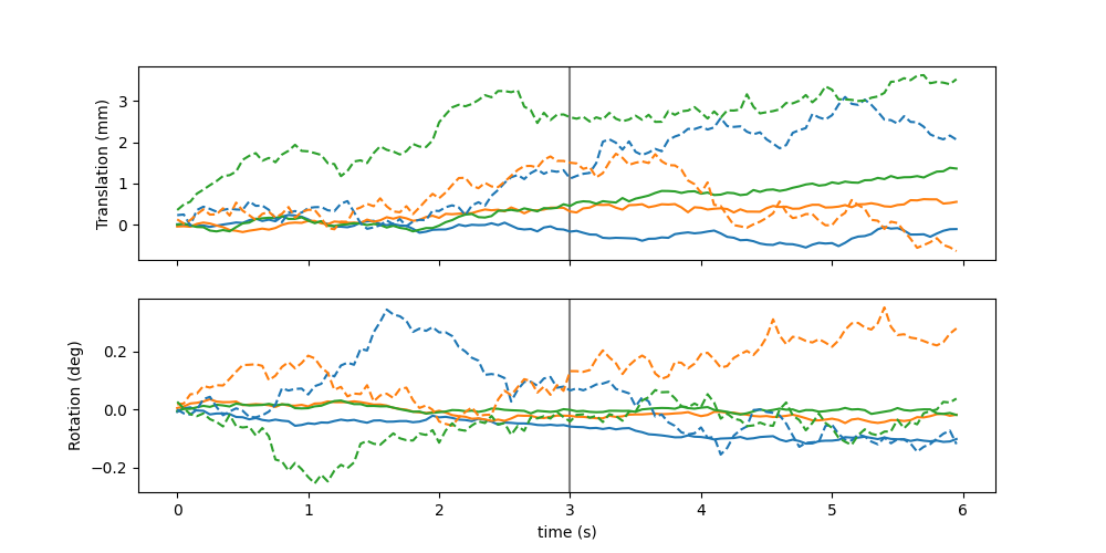
Show the motion#
fig, axs = plt.subplots(2, 1, figsize=(10, 5), sharex=True)
time = np.arange(len(motion.data[0])) * sim_conf.seq.TR / 1000
TR_vol = 3  # We generated 2 frames in 6 seconds
axs[0].axvline(TR_vol, c="gray")
axs[1].axvline(TR_vol, c="gray")


axs[0].plot(time, motion.data[:3, :].T)
axs[1].plot(time, motion.data[3:, :].T)
axs[0].set_prop_cycle(None)  # reset color cycling
axs[1].set_prop_cycle(None)
axs[0].plot(time, motion2.data[:3, :].T, linestyle="dashed")
axs[1].plot(time, motion2.data[3:, :].T, linestyle="dashed")

axs[1].set_xlabel("time (s)")
axs[0].set_ylabel("Translation (mm)")
axs[1].set_ylabel("Rotation (deg)")
Text(76.22222222222221, 0.5, 'Rotation (deg)')
Visualizing the reconstructed data#
import matplotlib.pyplot as plt

from snake.toolkit.plotting import axis3dcut

fig, axs = plt.subplots(1, 3, figsize=(26, 5))

axis3dcut(
    rec_motion[0].T,
    None,
    None,
    cbar=False,
    cuts=(0.5, 0.5, 0.5),
    ax=axs[0],
)
axis3dcut(
    rec_motion2[0].T,
    None,
    None,
    cbar=False,
    cuts=(0.5, 0.5, 0.5),
    ax=axs[1],
)
axis3dcut(rec_nomotion[0].T, None, None, cbar=False, cuts=(0.5, 0.5, 0.5), ax=axs[2])
axs[0].set_title("Small motion")
axs[1].set_title("Big motion")
axs[2].set_title("No motion")
plt.show()

/volatile/github-ci-mind-inria/gpu_mind_runner/_work/_tool/Python/3.10.16/x64/lib/python3.10/site-packages/numpy/lib/_function_base_impl.py:4620: RuntimeWarning: invalid value encountered in subtract
  diff_b_a = subtract(b, a)
sim_conf.seq.TR_eff
50
Total running time of the script: (1 minutes 15.219 seconds)