Note
Go to the end to download the full example code.
Measuring variable importance in classification#
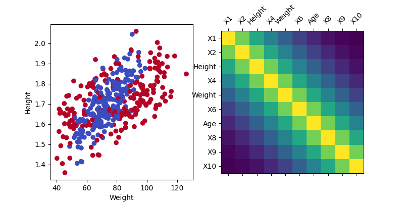
In this example, we illustrate how to measure variable importance in a classification context. The problem under consideration is a binary classification where the target variable is generated using a non-linear function of the features. Therefore illustrating the importance of model-agnostic variable importance methods, which, as opposed to linear models for instance, can capture non-linear relationships. The features are generated from a multivariate normal distribution with a Toeplitz correlation matrix. This second specificity of the problem is interesting to exemplify the benefits of the conditional permutation importance (CPI) method [CHAMMA et al.[1]] over the standard permutation importance (PI) method [Breiman[2]].
References#
Imports needed#
import matplotlib.lines as mlines
import matplotlib.pyplot as plt
import numpy as np
from scipy.linalg import toeplitz
from scipy.stats import ttest_1samp
from sklearn.base import clone
from sklearn.linear_model import RidgeCV
from sklearn.metrics import hinge_loss
from sklearn.model_selection import RandomizedSearchCV, StratifiedKFold
from sklearn.svm import SVC

from hidimstat import CPI, PermutationImportance
Generate the data#
We generate the data using a multivariate normal distribution with a Toeplitz correlation matrix. The target variable is generated using a non-linear function of the features. To make the problem more intuitive, we generate a non-linear combination of the features inspired by the Body Mass Index (BMI) formula. The BMI can be obtained by \(\text{BMI} = \frac{\text{weight}}{\text{height}^2}\). And we simply mimic the weight and height variables by rescaling 2 correlated features. The binary target is then generated using the formula: \(y = \beta_1 \exp\left(\frac{|\text{bmi} - \text{mean(bmi)}|}{\text{std(bmi)}} \right) + \beta_2 \exp\left(|\text{weight}| \times 1\left[|\text{weight} - \text{mean(weight)}| > \text{quantile(weight, 0.80)}\right] \right) + \beta_3 \cdot \text{age} + \epsilon\) where \(\epsilon`\) is a Gaussian noise. The first and second term are non-linear functions of the features, corresponding to deviations from the population mean while the third term is a linear function of a feature.
seed = 0
rng = np.random.RandomState(seed)
n_samples = 400
n_features = 10
corr_mat = toeplitz(
    np.linspace(1, 0.0, n_features) ** 2,
)
mean = np.zeros(corr_mat.shape[0])
X = rng.multivariate_normal(
    mean,
    corr_mat,
    size=n_samples,
)
noise_y = 0.5
weight = X[:, 4] * 20 + 74
weight[weight < 40] += 30
height = X[:, 2] * 0.12 + 1.7
age = X[:, 6] * 10 + 50
bmi = weight / height**2

a = np.exp(np.abs(bmi - np.mean(bmi)) / np.std(bmi))
b = np.exp(
    np.abs(X[:, 4])
    * ((X[:, 4] < np.quantile(X[:, 4], 0.10)) + (X[:, 4] > np.quantile(X[:, 4], 0.90)))
)

y_cont = 4 * a + 2.0 * b + 0.5 * age + noise_y * rng.randn(n_samples)
y = y_cont > np.quantile(y_cont, 0.5)
Visualize the data#
fig, axes = plt.subplots(
    1,
    2,
    figsize=(8, 4),
)
axes[0].scatter(weight, height, c=y, cmap="coolwarm")
axes[0].set_xlabel("Weight")
axes[0].set_ylabel("Height")
axes[1].matshow(
    corr_mat,
)
labels = np.array(
    [
        "X1",
        "X2",
        "Height",
        "X4",
        "Weight",
        "X6",
        "Age",
        "X8",
        "X9",
        "X10",
    ]
)
tck_ids = np.arange(0, n_features)
axes[1].set_xticks(tck_ids, labels[tck_ids], rotation=45)
axes[1].set_yticks(tck_ids, labels[tck_ids])

[<matplotlib.axis.YTick object at 0x7f85761a6ab0>, <matplotlib.axis.YTick object at 0x7f8581419520>, <matplotlib.axis.YTick object at 0x7f858e814c20>, <matplotlib.axis.YTick object at 0x7f858e8165d0>, <matplotlib.axis.YTick object at 0x7f858e814a10>, <matplotlib.axis.YTick object at 0x7f858e8165a0>, <matplotlib.axis.YTick object at 0x7f858e8162a0>, <matplotlib.axis.YTick object at 0x7f858ea6f230>, <matplotlib.axis.YTick object at 0x7f858ea6de80>, <matplotlib.axis.YTick object at 0x7f858e8148c0>]
Variable importance inference#
We use two different Support Vector Machine models, one with a linear kernel and one with a polynomial kernel of degree 2, well specified to capture the non-linear relationship between the features and the target variable. We then use the CPI and PI methods to compute the variable importance. We use a 5-fold cross-validation to estimate the importance of the features.
seed = 0
cv = StratifiedKFold(n_splits=5, shuffle=True, random_state=seed)
importance_linear = []
importance_non_linear = []
important_pi = []

model_linear = RandomizedSearchCV(
    SVC(random_state=seed, kernel="linear"),
    param_distributions={
        "C": np.logspace(-3, 3, 10),
    },
    n_iter=10,
    n_jobs=5,
    random_state=seed,
)
model_non_linear = RandomizedSearchCV(
    SVC(
        random_state=seed,
        kernel="poly",
        degree=2,
        coef0=1,
    ),
    param_distributions={
        "C": np.logspace(-3, 3, 10),
    },
    n_iter=10,
    n_jobs=5,
    random_state=seed,
)
imputation_model = RidgeCV(alphas=np.logspace(-3, 3, 50))


importance_list = []
for train, test in cv.split(X, y):
    model_linear_c = clone(model_linear)
    model_linear_c.fit(X[train], y[train])
    cpi_linear = CPI(
        estimator=model_linear_c,
        imputation_model_continuous=clone(imputation_model),
        n_permutations=50,
        n_jobs=5,
        loss=hinge_loss,
        random_state=seed,
        method="decision_function",
    )
    cpi_linear.fit(X[train], y[train])
    imp_cpi_linear = cpi_linear.score(X[test], y[test])["importance"]

    model_non_linear_c = clone(model_non_linear)
    model_non_linear_c.fit(X[train], y[train])
    cpi_non_linear = CPI(
        estimator=model_non_linear_c,
        imputation_model_continuous=clone(imputation_model),
        n_permutations=50,
        n_jobs=5,
        loss=hinge_loss,
        random_state=seed,
        method="decision_function",
    )
    cpi_non_linear.fit(X[train], y[train])
    imp_cpi_non_linear = cpi_non_linear.score(X[test], y[test])["importance"]

    pi_non_linear = PermutationImportance(
        estimator=model_non_linear_c,
        n_permutations=50,
        n_jobs=5,
        random_state=seed,
        method="decision_function",
    )
    pi_non_linear.fit(X[train], y[train])
    imp_pi_non_linear = pi_non_linear.score(X[test], y[test])["importance"]

    importance_list.append(
        np.stack(
            [
                imp_cpi_linear,
                imp_cpi_non_linear,
                imp_pi_non_linear,
            ]
        )
    )

importance_arr = np.stack(importance_list)
Compute the p-values for the variable importance#
pval_arr = np.zeros((n_features, 3))
for j in range(n_features):
    for i in range(3):
        diff = importance_arr[:, i, j]
        pval_arr[j, i] = ttest_1samp(diff, 0)[1]
Visualize the variable importance#
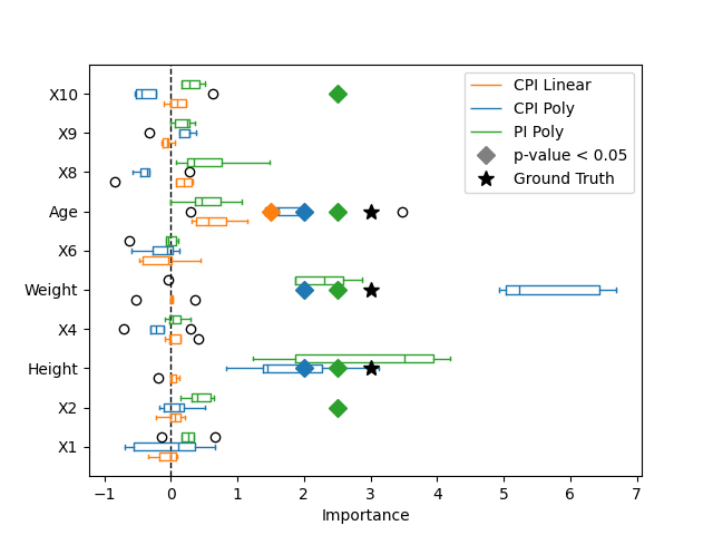
Here we plot the variable importance and highlight the features that are considered important, with a p-value lower than 0.05, using a diamond marker. We also highlight the true important features, used to generate the target variable, with a star marker. While the linear model captures the importance of the age, it fails to capture the importance of the weight and height because of its lack of expressivity. Using a polynomial kernel, the non-linear model captures the importance of the weight and height. Finally, the CPI method controls for false positive discoveries contrarily to the PI method which identifies spurious important features simply because of the correlation structure of the features.
fig, ax = plt.subplots()
box1 = ax.boxplot(
    importance_arr[:, 0, :],
    positions=np.arange(1, n_features + 1) - 0.25,
    widths=0.2,
    label="CPI Linear",
    vert=False,
)
for item in ["whiskers", "fliers", "medians", "caps", "boxes"]:
    plt.setp(box1[item], color="tab:orange")

box1 = ax.boxplot(
    importance_arr[:, 1, :],
    positions=np.arange(1, n_features + 1),
    widths=0.2,
    label="CPI Poly",
    vert=False,
)
for item in ["whiskers", "fliers", "medians", "caps", "boxes"]:
    plt.setp(box1[item], color="tab:blue")

box1 = ax.boxplot(
    importance_arr[:, 2, :],
    positions=np.arange(1, n_features + 1) + 0.25,
    widths=0.2,
    label="PI Poly",
    vert=False,
)
for item in ["whiskers", "fliers", "medians", "caps", "boxes"]:
    plt.setp(box1[item], color="tab:green")

ax.set_yticks(np.arange(1, n_features + 1), labels)
ax.legend()
ax.axvline(0, color="black", lw=1, ls="--", zorder=-1)
ax.set_xlabel("Importance")

# Plot the important features based on thresholded p-values
threshold = 0.05
for j in range(n_features):
    for i, color in enumerate(["tab:orange", "tab:blue", "tab:green"]):

        if pval_arr[j, i] < threshold:
            ax.plot(
                2 + (i - 1) * 0.5,
                j + 1,
                marker="D",
                color=color,
                markersize=8,
                zorder=3,
            )
    if j in [2, 4, 6]:
        ax.plot(
            3,
            j + 1,
            marker="*",
            color="k",
            markersize=10,
            zorder=3,
        )
important_legend = mlines.Line2D(
    [],
    [],
    color="grey",
    marker="D",
    linestyle="None",
    markersize=8,
    label=f"p-value < {threshold}",
)
ground_truth_legend = mlines.Line2D(
    [], [], color="k", marker="*", linestyle="None", markersize=10, label="Ground Truth"
)
handles = ax.get_legend_handles_labels()[0]
ax.legend(handles=handles + [important_legend, ground_truth_legend], loc="upper right")

<matplotlib.legend.Legend object at 0x7f85808f51c0>
Total running time of the script: (0 minutes 32.118 seconds)
Estimated memory usage: 193 MB
