
Note
Go to the end to download the full example code or to run this example in your browser via Binder.
Least Squares Image Reconstruction#
An example to show how to reconstruct volumes using the least square estimate.
This script demonstrates the use of the Conjugate Gradient (CG), LSQR and LSMR methods, to reconstruct images from non-uniform k-space data.
import os
import time
from tqdm.auto import tqdm
import cupy as cp
import numpy as np
from brainweb_dl import get_mri
from matplotlib import pyplot as plt
from skimage.metrics import peak_signal_noise_ratio as psnr

import mrinufft
from mrinufft.extras import loss_l2_reg, loss_l2_AHreg
from mrinufft.trajectories import initialize_2D_spiral

BACKEND = os.environ.get("MRINUFFT_BACKEND", "cufinufft")
Setup Inputs
samples_loc = initialize_2D_spiral(Nc=64, Ns=512, nb_revolutions=8)
ground_truth = get_mri(sub_id=4)
ground_truth = ground_truth[90]
# Normalize the ground truth image
ground_truth = ground_truth / np.sqrt(np.mean(abs(ground_truth) ** 2))
image_gpu = cp.array(ground_truth)  # convert to cupy array for GPU processing

print("image size: ", ground_truth.shape)
image size: (256, 256)
Setup the NUFFT operator
NufftOperator = mrinufft.get_operator(BACKEND)  # get the operator

nufft = NufftOperator(
    samples_loc,
    shape=ground_truth.shape,
    squeeze_dims=True,
)  # create the NUFFT operator
Reconstruct the image using the CG method
kspace_data_gpu = nufft.op(image_gpu)  # get the k-space data
kspace_data = kspace_data_gpu.get()  # convert back to numpy array for display
adjoint = nufft.adj_op(kspace_data_gpu).get()  # adjoint NUFFT
/volatile/github-ci-mind-inria/gpu_mind_runner/_work/mri-nufft/mri-nufft/.venv/lib/python3.12/site-packages/cufinufft/_plan.py:402: UserWarning: Argument `data` does not satisfy the following requirement: C. Copying array (this may reduce performance)
  warnings.warn(f"Argument `{name}` does not satisfy the "
Pseudo-inverse solver#
The least-square solution to the inverse problem can be obtained by solving the following optimization problem:
where \(A\) is the NUFFT operator, \(x\) is the image to be
reconstructed, and \(b\) is the k-space data. The optimization problem can
be solved using different iterative solvers, such as Conjugate Gradient (CG),
LSQR and LSMR. The solvers are implemented in the mrinufft.pinv_solver()
method, which takes as input the k-space data, the maximum number of
iterations, and the optimization method to use.
Callback monitoring#
We can monitor the convergence of the optimization by using a callback function that is called at each iteration of the optimization. The callback function can compute different metrics, such as the residual norm, the PSNR, or the time taken
def mixed_cb(*args, **kwargs):
    """A compound callback function, to track iterations time and convergence."""
    return [
        time.perf_counter(),
        loss_l2_reg(*args, **kwargs),
        loss_l2_AHreg(*args, **kwargs),
        psnr(
            abs(args[0].get().squeeze()),
            abs(ground_truth.squeeze()),
            data_range=ground_truth.max(),
        ),
        time.perf_counter(),
    ]


def process_cb_results(cb_results):
    t0, r, rH, psnrs, t1 = list(zip(*cb_results))
    t1 = (t0[0], *t1[:-1])
    time_it = np.cumsum(np.array(t0) - np.array(t1))
    r = [rr.get() for rr in r]
    rH = [rr.get() for rr in rH]

    return {"time": time_it, "res": r, "AHres": rH, "psnr": psnrs}
Run the least-square minimization for all the solvers#
OPTIM = ["cg", "lsqr", "lsmr"]
METRICS = {
    "res": r"$\|Ax-b\|$",
    "AHres": r"$\|A^H(Ax-b)\|$",
    "psnr": "PSNR",
}

MAX_ITER = 1000

images = dict()
iterations_cb = dict()
pg = tqdm(total=MAX_ITER, position=0, leave=True)
for optim in OPTIM:
    image, iter_cb = nufft.pinv_solver(
        kspace_data=kspace_data_gpu,
        max_iter=MAX_ITER,
        callback=mixed_cb,
        optim=optim,
        progressbar=pg,
    )
    images[optim] = image.get().squeeze()  # retrieve image from GPU.
    iterations_cb[optim] = process_cb_results(iter_cb)
  0%|          | 0/1000 [00:00<?, ?it/s]
  0%|          | 0/1000 [00:00<?, ?it/s]
  1%|          | 12/1000 [00:00<00:08, 114.00it/s]
  2%|▏         | 24/1000 [00:00<00:08, 112.65it/s]
  4%|▍         | 38/1000 [00:00<00:07, 123.34it/s]
  5%|▌         | 51/1000 [00:00<00:08, 106.91it/s]
  6%|▌         | 62/1000 [00:00<00:09, 103.21it/s]
  7%|▋         | 74/1000 [00:00<00:08, 107.59it/s]
  9%|▉         | 88/1000 [00:00<00:07, 116.54it/s]
 10%|█         | 100/1000 [00:00<00:08, 100.32it/s]
 11%|█         | 111/1000 [00:01<00:09, 94.01it/s]
 12%|█▏        | 124/1000 [00:01<00:08, 102.66it/s]
 14%|█▍        | 140/1000 [00:01<00:07, 117.45it/s]
 16%|█▌        | 156/1000 [00:01<00:06, 128.73it/s]
 17%|█▋        | 170/1000 [00:01<00:06, 124.85it/s]
 18%|█▊        | 183/1000 [00:01<00:06, 124.88it/s]
 20%|█▉        | 196/1000 [00:01<00:06, 116.13it/s]
 21%|██        | 208/1000 [00:01<00:06, 113.52it/s]
 22%|██▏       | 220/1000 [00:01<00:07, 107.94it/s]
 23%|██▎       | 231/1000 [00:02<00:07, 102.84it/s]
 24%|██▍       | 242/1000 [00:02<00:07, 102.93it/s]
 26%|██▌       | 256/1000 [00:02<00:06, 110.28it/s]
 27%|██▋       | 272/1000 [00:02<00:05, 123.61it/s]
 28%|██▊       | 285/1000 [00:02<00:06, 105.88it/s]
 30%|██▉       | 297/1000 [00:02<00:06, 102.47it/s]
 31%|███       | 310/1000 [00:02<00:06, 106.59it/s]
 32%|███▏      | 324/1000 [00:02<00:05, 113.69it/s]
 34%|███▍      | 338/1000 [00:03<00:05, 120.18it/s]
 35%|███▌      | 351/1000 [00:03<00:05, 116.57it/s]
 36%|███▋      | 363/1000 [00:03<00:05, 117.00it/s]
 38%|███▊      | 377/1000 [00:03<00:05, 121.09it/s]
 39%|███▉      | 390/1000 [00:03<00:05, 118.88it/s]
 40%|████      | 402/1000 [00:03<00:05, 116.93it/s]
 41%|████▏     | 414/1000 [00:03<00:05, 112.31it/s]
 43%|████▎     | 426/1000 [00:03<00:05, 105.45it/s]
 44%|████▎     | 437/1000 [00:03<00:05, 105.85it/s]
 45%|████▍     | 449/1000 [00:04<00:05, 109.55it/s]
 46%|████▌     | 461/1000 [00:04<00:04, 108.06it/s]
 47%|████▋     | 472/1000 [00:04<00:05, 100.65it/s]
 48%|████▊     | 483/1000 [00:04<00:05, 99.48it/s]
 50%|████▉     | 497/1000 [00:04<00:04, 109.78it/s]
 51%|█████▏    | 514/1000 [00:04<00:03, 124.47it/s]
 53%|█████▎    | 529/1000 [00:04<00:03, 127.93it/s]
 54%|█████▍    | 542/1000 [00:04<00:03, 118.03it/s]
 56%|█████▌    | 557/1000 [00:04<00:03, 126.22it/s]
 57%|█████▋    | 571/1000 [00:05<00:03, 129.51it/s]
 59%|█████▊    | 586/1000 [00:05<00:03, 132.53it/s]
 60%|██████    | 600/1000 [00:05<00:03, 126.41it/s]
 61%|██████▏   | 613/1000 [00:05<00:03, 123.60it/s]
 63%|██████▎   | 629/1000 [00:05<00:02, 131.80it/s]
 65%|██████▍   | 646/1000 [00:05<00:02, 140.02it/s]
 66%|██████▌   | 661/1000 [00:05<00:02, 140.17it/s]
 68%|██████▊   | 676/1000 [00:05<00:02, 126.78it/s]
 69%|██████▉   | 691/1000 [00:05<00:02, 130.11it/s]
 70%|███████   | 705/1000 [00:06<00:02, 131.82it/s]
 72%|███████▏  | 720/1000 [00:06<00:02, 135.63it/s]
 73%|███████▎  | 734/1000 [00:06<00:02, 127.59it/s]
 75%|███████▍  | 747/1000 [00:06<00:02, 124.34it/s]
 76%|███████▋  | 763/1000 [00:06<00:01, 133.09it/s]
 78%|███████▊  | 779/1000 [00:06<00:01, 138.14it/s]
 79%|███████▉  | 794/1000 [00:06<00:01, 138.71it/s]
 81%|████████  | 808/1000 [00:06<00:01, 121.75it/s]
 82%|████████▏ | 823/1000 [00:06<00:01, 125.69it/s]
 84%|████████▎ | 837/1000 [00:07<00:01, 129.32it/s]
 85%|████████▌ | 852/1000 [00:07<00:01, 134.20it/s]
 87%|████████▋ | 866/1000 [00:07<00:01, 124.60it/s]
 88%|████████▊ | 880/1000 [00:07<00:00, 126.83it/s]
 90%|████████▉ | 895/1000 [00:07<00:00, 131.92it/s]
 91%|█████████ | 911/1000 [00:07<00:00, 138.68it/s]
 93%|█████████▎| 926/1000 [00:07<00:00, 134.08it/s]
 94%|█████████▍| 940/1000 [00:07<00:00, 129.64it/s]
 96%|█████████▌| 955/1000 [00:07<00:00, 132.85it/s]
 97%|█████████▋| 969/1000 [00:08<00:00, 133.86it/s]
 98%|█████████▊| 984/1000 [00:08<00:00, 136.62it/s]
100%|█████████▉| 998/1000 [00:08<00:00, 122.53it/s]
  0%|          | 0/1000 [00:00<?, ?it/s]
  1%|▏         | 13/1000 [00:00<00:10, 93.74it/s]
  2%|▎         | 25/1000 [00:00<00:09, 103.78it/s]
  4%|▎         | 36/1000 [00:00<00:11, 82.31it/s]
  5%|▍         | 47/1000 [00:00<00:10, 88.29it/s]
  6%|▌         | 57/1000 [00:00<00:10, 91.74it/s]
  7%|▋         | 68/1000 [00:00<00:09, 95.63it/s]
  8%|▊         | 78/1000 [00:00<00:10, 85.55it/s]
  9%|▊         | 87/1000 [00:00<00:10, 86.14it/s]
 10%|▉         | 98/1000 [00:01<00:09, 91.84it/s]
 11%|█         | 110/1000 [00:01<00:08, 99.26it/s]
 12%|█▏        | 121/1000 [00:01<00:08, 100.90it/s]
 13%|█▎        | 132/1000 [00:01<00:08, 100.34it/s]
 14%|█▍        | 143/1000 [00:01<00:10, 85.20it/s]
 15%|█▌        | 154/1000 [00:01<00:09, 90.48it/s]
 17%|█▋        | 166/1000 [00:01<00:08, 96.34it/s]
 18%|█▊        | 177/1000 [00:01<00:08, 94.69it/s]
 19%|█▊        | 187/1000 [00:02<00:09, 83.62it/s]
 20%|█▉        | 198/1000 [00:02<00:08, 89.90it/s]
 21%|██        | 209/1000 [00:02<00:08, 94.89it/s]
 22%|██▏       | 220/1000 [00:02<00:07, 98.52it/s]
 23%|██▎       | 231/1000 [00:02<00:09, 83.93it/s]
 24%|██▍       | 242/1000 [00:02<00:08, 88.84it/s]
 25%|██▌       | 253/1000 [00:02<00:08, 93.21it/s]
 26%|██▋       | 264/1000 [00:02<00:07, 96.85it/s]
 27%|██▋       | 274/1000 [00:03<00:08, 84.61it/s]
 28%|██▊       | 285/1000 [00:03<00:08, 89.20it/s]
 30%|██▉       | 296/1000 [00:03<00:07, 92.48it/s]
 31%|███       | 306/1000 [00:03<00:07, 93.83it/s]
 32%|███▏      | 316/1000 [00:03<00:07, 95.09it/s]
 33%|███▎      | 326/1000 [00:03<00:08, 82.31it/s]
 34%|███▎      | 337/1000 [00:03<00:07, 88.37it/s]
 35%|███▍      | 347/1000 [00:03<00:07, 91.31it/s]
 36%|███▌      | 359/1000 [00:03<00:06, 96.98it/s]
 37%|███▋      | 369/1000 [00:04<00:07, 84.20it/s]
 38%|███▊      | 379/1000 [00:04<00:07, 86.98it/s]
 39%|███▉      | 390/1000 [00:04<00:06, 92.23it/s]
 40%|████      | 400/1000 [00:04<00:06, 93.33it/s]
 41%|████      | 410/1000 [00:04<00:06, 94.24it/s]
 42%|████▏     | 420/1000 [00:04<00:07, 82.46it/s]
 43%|████▎     | 432/1000 [00:04<00:06, 90.48it/s]
 44%|████▍     | 444/1000 [00:04<00:05, 97.31it/s]
 46%|████▌     | 455/1000 [00:04<00:05, 99.96it/s]
 47%|████▋     | 466/1000 [00:05<00:06, 83.29it/s]
 48%|████▊     | 477/1000 [00:05<00:05, 88.28it/s]
 49%|████▉     | 488/1000 [00:05<00:05, 92.34it/s]
  0%|          | 0/1000 [00:00<?, ?it/s]
  1%|          | 10/1000 [00:00<00:13, 74.85it/s]
  2%|▏         | 18/1000 [00:00<00:16, 57.91it/s]
  3%|▎         | 28/1000 [00:00<00:13, 71.10it/s]
  4%|▍         | 38/1000 [00:00<00:12, 80.05it/s]
  5%|▍         | 48/1000 [00:00<00:11, 84.91it/s]
  6%|▌         | 57/1000 [00:00<00:13, 70.17it/s]
  6%|▋         | 65/1000 [00:00<00:13, 70.73it/s]
  7%|▋         | 74/1000 [00:01<00:12, 73.62it/s]
  8%|▊         | 84/1000 [00:01<00:11, 79.92it/s]
  9%|▉         | 93/1000 [00:01<00:12, 71.37it/s]
 10%|█         | 101/1000 [00:01<00:12, 72.69it/s]
 11%|█         | 111/1000 [00:01<00:11, 78.77it/s]
 12%|█▏        | 121/1000 [00:01<00:10, 82.62it/s]
 13%|█▎        | 130/1000 [00:01<00:10, 82.44it/s]
 14%|█▍        | 139/1000 [00:01<00:12, 69.48it/s]
 15%|█▍        | 147/1000 [00:01<00:11, 71.88it/s]
 16%|█▌        | 157/1000 [00:02<00:10, 77.22it/s]
 17%|█▋        | 166/1000 [00:02<00:10, 78.32it/s]
 18%|█▊        | 175/1000 [00:02<00:11, 69.90it/s]
 19%|█▊        | 186/1000 [00:02<00:10, 78.40it/s]
 20%|█▉        | 195/1000 [00:02<00:10, 80.06it/s]
 20%|██        | 204/1000 [00:02<00:09, 80.07it/s]
 21%|██▏       | 213/1000 [00:02<00:11, 68.36it/s]
 22%|██▏       | 221/1000 [00:02<00:11, 70.79it/s]
 23%|██▎       | 231/1000 [00:03<00:09, 78.07it/s]
 24%|██▍       | 240/1000 [00:03<00:09, 78.39it/s]
 25%|██▍       | 249/1000 [00:03<00:10, 71.79it/s]
 26%|██▌       | 258/1000 [00:03<00:09, 75.40it/s]
 27%|██▋       | 268/1000 [00:03<00:09, 79.28it/s]
 28%|██▊       | 277/1000 [00:03<00:08, 81.82it/s]
 29%|██▊       | 286/1000 [00:03<00:08, 81.18it/s]
 30%|██▉       | 295/1000 [00:03<00:10, 68.16it/s]
 30%|███       | 305/1000 [00:04<00:09, 75.35it/s]
 32%|███▏      | 315/1000 [00:04<00:08, 79.89it/s]
 32%|███▎      | 325/1000 [00:04<00:07, 84.86it/s]
 33%|███▎      | 334/1000 [00:04<00:09, 73.65it/s]
 34%|███▍      | 343/1000 [00:04<00:08, 75.73it/s]
 35%|███▌      | 352/1000 [00:04<00:08, 79.33it/s]
 36%|███▌      | 361/1000 [00:04<00:07, 79.88it/s]
 37%|███▋      | 370/1000 [00:04<00:09, 68.25it/s]
 38%|███▊      | 379/1000 [00:05<00:08, 73.43it/s]
 39%|███▉      | 388/1000 [00:05<00:07, 77.30it/s]
 40%|███▉      | 398/1000 [00:05<00:07, 83.28it/s]
 41%|████      | 408/1000 [00:05<00:06, 86.57it/s]
 42%|████▏     | 417/1000 [00:05<00:08, 70.69it/s]
 43%|████▎     | 426/1000 [00:05<00:07, 74.87it/s]
 44%|████▎     | 435/1000 [00:05<00:07, 77.17it/s]
 44%|████▍     | 444/1000 [00:05<00:07, 78.91it/s]
 45%|████▌     | 453/1000 [00:06<00:07, 68.45it/s]
 46%|████▋     | 463/1000 [00:06<00:07, 75.52it/s]
 47%|████▋     | 473/1000 [00:06<00:06, 81.03it/s]
 48%|████▊     | 483/1000 [00:06<00:06, 85.77it/s]
 49%|████▉     | 492/1000 [00:06<00:07, 71.36it/s]
 50%|█████     | 501/1000 [00:06<00:06, 74.46it/s]
 51%|█████     | 510/1000 [00:06<00:06, 75.97it/s]
 52%|█████▏    | 519/1000 [00:06<00:06, 78.37it/s]
 53%|█████▎    | 528/1000 [00:06<00:06, 74.98it/s]
 54%|█████▎    | 536/1000 [00:07<00:06, 71.40it/s]
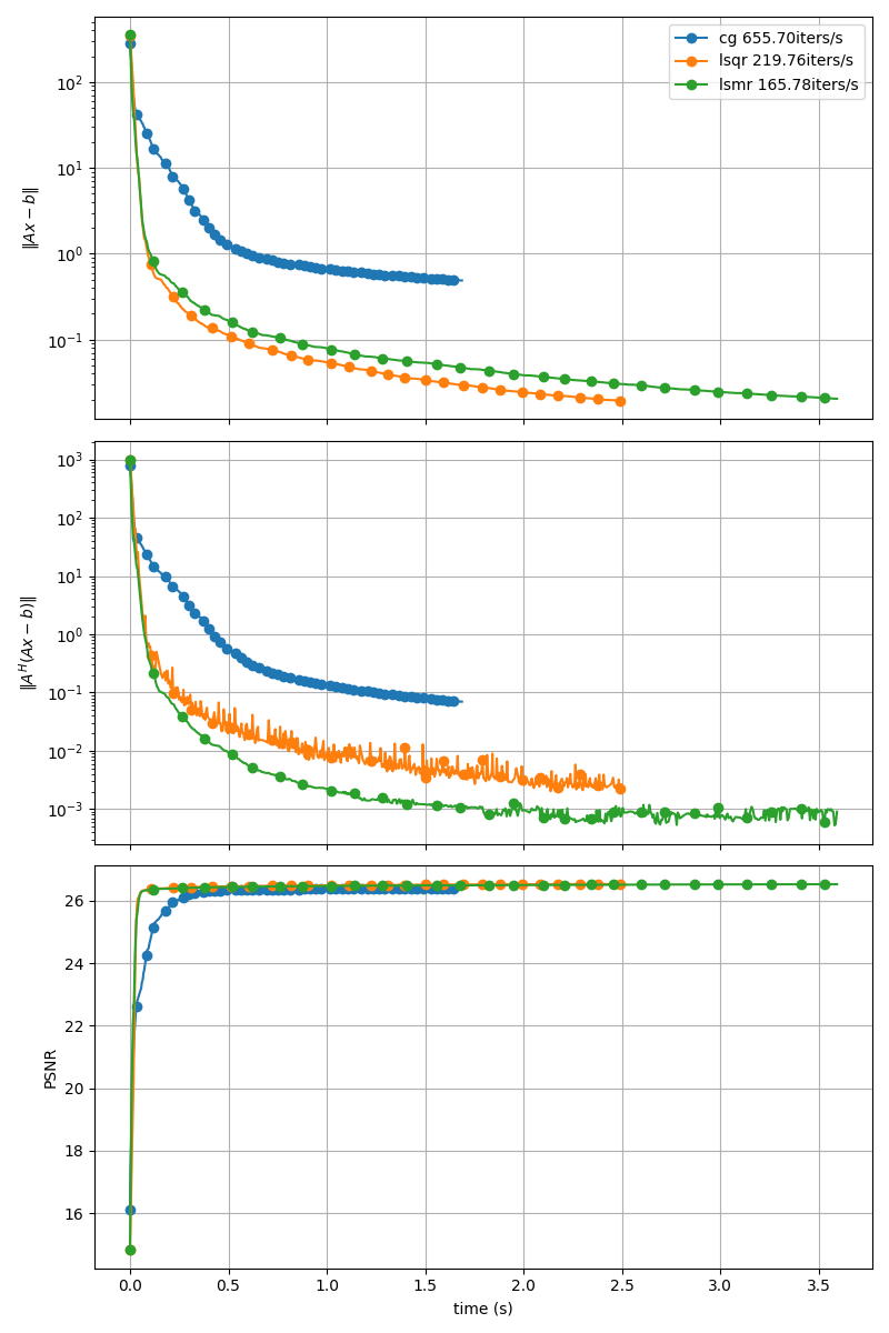
Display Convergence#
fig, axs = plt.subplots(len(METRICS), 1, sharex=True, figsize=(8, 12))
for i, metric in enumerate(METRICS):
    for optim in OPTIM:
        if "res" in metric:
            axs[i].set_yscale("log")
        axs[i].plot(
            iterations_cb[optim]["time"],
            iterations_cb[optim][metric],
            marker="o",
            markevery=20,
            label=f"{optim} {np.mean(1/np.diff(iterations_cb[optim]['time'])):.2f}iters/s",
        )
    axs[i].grid()
    axs[i].set_ylabel(METRICS[metric])
axs[0].legend()
axs[-1].set_xlabel("time (s)")
fig.tight_layout()
plt.show()
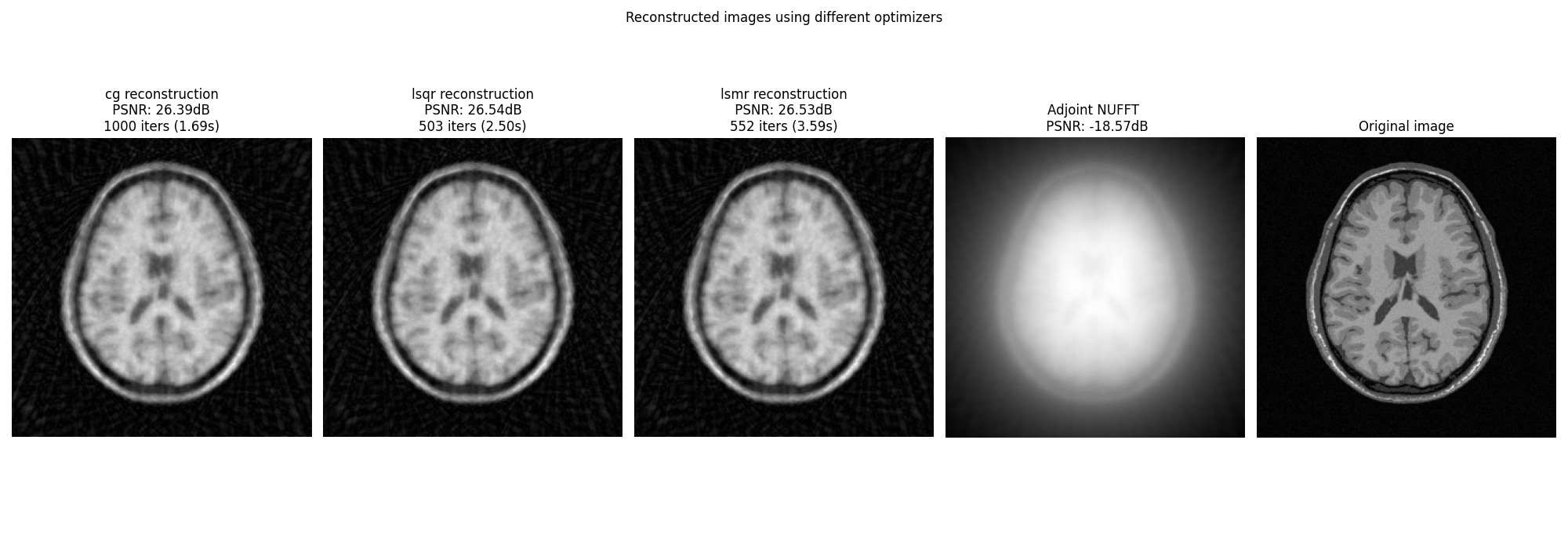
Display images#
fig, axs = plt.subplots(1, len(OPTIM) + 2, figsize=(20, 7))

for i, optim in enumerate(OPTIM):
    axs[i].imshow(abs(images[optim]), cmap="gray", origin="lower")
    axs[i].axis("off")
    axs[i].set_title(
        f"{optim} reconstruction\n PSNR: {iterations_cb[optim]['psnr'][-1]:.2f}dB \n"
        f"{len(iterations_cb[optim]['time'])} iters ({iterations_cb[optim]['time'][-1]:.2f}s)"
    )

axs[-1].imshow(abs(ground_truth), cmap="gray", origin="lower")
axs[-1].axis("off")
axs[-1].set_title("Original image")
axs[-2].imshow(
    abs(adjoint),
    cmap="gray",
    origin="lower",
)
axs[-2].axis("off")
axs[-2].set_title(
    f"Adjoint NUFFT \n PSNR: {psnr(abs(adjoint), abs(ground_truth), data_range=ground_truth.max()):.2f}dB"
)

fig.suptitle("Reconstructed images using different optimizers")
fig.tight_layout()
plt.show()
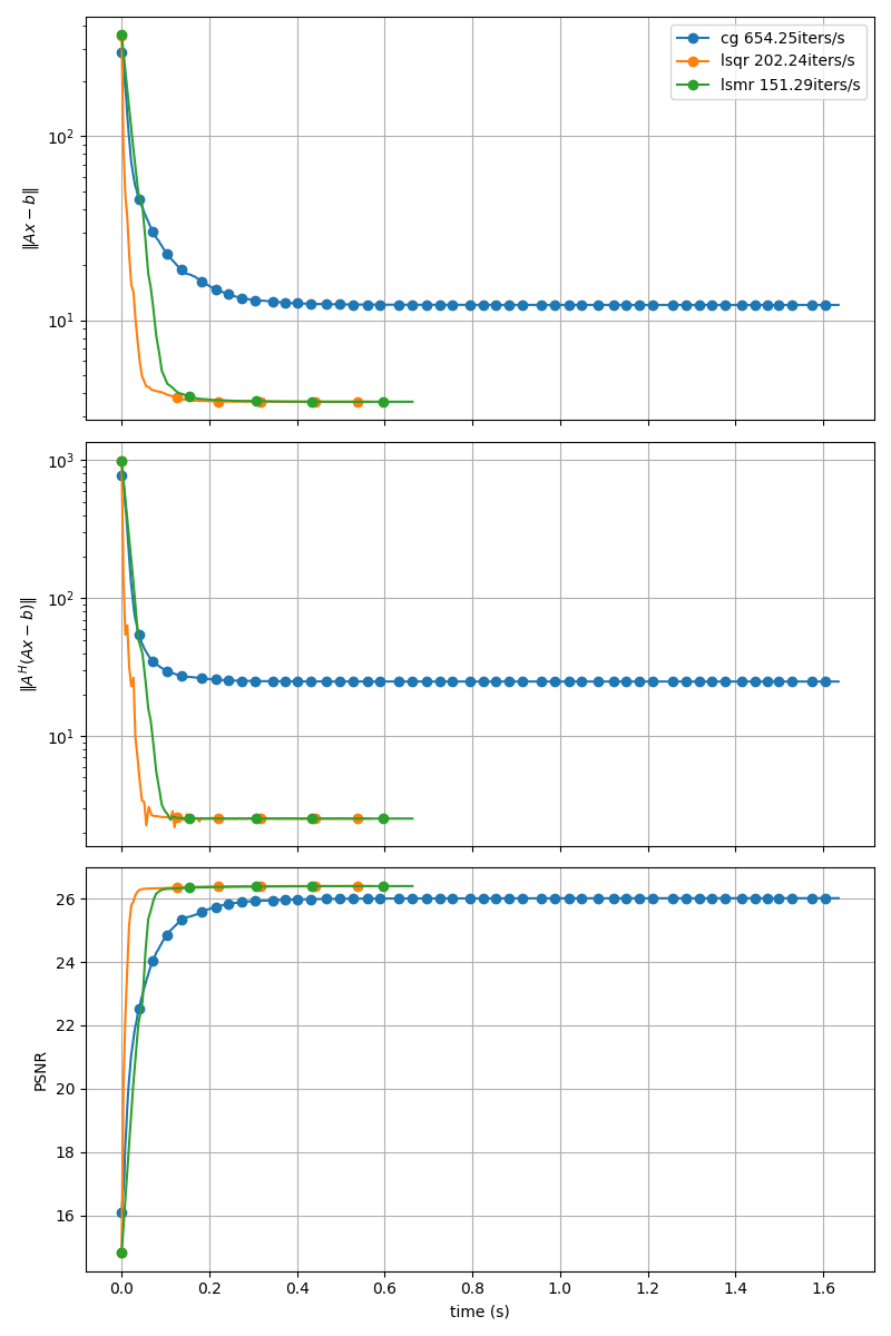
Using a damping regularization term#
The least-square problem can be regularized using a damping term to improve the conditioning of the problem. This is done by solving the following optimization problem:
#    \min_x \|Ax - b\|_2^2 + \gamma \|x\|_2^2

# where :math:`\gamma` is the regularization parameter.


images = dict()
iterations_cb = dict()

pg = tqdm(total=MAX_ITER, position=0, leave=True)
for optim in OPTIM:
    image, iter_cb = nufft.pinv_solver(
        kspace_data=kspace_data_gpu,
        max_iter=1000,
        callback=mixed_cb,
        damp=0.1,
        optim=optim,
        progressbar=pg,
    )
    images[optim] = image.get().squeeze()  # retrieve image from GPU.
    iterations_cb[optim] = process_cb_results(iter_cb)
  0%|          | 0/1000 [00:00<?, ?it/s]
 54%|█████▎    | 537/1000 [00:08<00:07, 60.85it/s]

  0%|          | 0/1000 [00:00<?, ?it/s]
  2%|▏         | 15/1000 [00:00<00:06, 147.65it/s]
  3%|▎         | 30/1000 [00:00<00:08, 119.77it/s]
  4%|▍         | 45/1000 [00:00<00:07, 129.36it/s]
  6%|▌         | 59/1000 [00:00<00:07, 131.83it/s]
  7%|▋         | 73/1000 [00:00<00:07, 132.18it/s]
  9%|▊         | 87/1000 [00:00<00:07, 129.32it/s]
 10%|█         | 101/1000 [00:00<00:07, 119.15it/s]
 12%|█▏        | 116/1000 [00:00<00:07, 125.61it/s]
 13%|█▎        | 132/1000 [00:01<00:06, 133.69it/s]
 15%|█▍        | 148/1000 [00:01<00:06, 139.40it/s]
 16%|█▋        | 163/1000 [00:01<00:05, 140.18it/s]
 18%|█▊        | 178/1000 [00:01<00:06, 126.70it/s]
 19%|█▉        | 192/1000 [00:01<00:06, 128.59it/s]
 21%|██        | 206/1000 [00:01<00:06, 128.42it/s]
 22%|██▏       | 220/1000 [00:01<00:06, 129.62it/s]
 24%|██▎       | 235/1000 [00:01<00:05, 135.10it/s]
 25%|██▍       | 249/1000 [00:01<00:06, 121.01it/s]
 26%|██▋       | 265/1000 [00:02<00:05, 130.03it/s]
 28%|██▊       | 281/1000 [00:02<00:05, 137.17it/s]
 30%|██▉       | 297/1000 [00:02<00:05, 140.57it/s]
 31%|███       | 312/1000 [00:02<00:04, 138.19it/s]
 33%|███▎      | 326/1000 [00:02<00:05, 123.29it/s]
 34%|███▍      | 339/1000 [00:02<00:05, 123.08it/s]
 35%|███▌      | 354/1000 [00:02<00:05, 128.23it/s]
 37%|███▋      | 369/1000 [00:02<00:04, 133.57it/s]
 38%|███▊      | 383/1000 [00:02<00:04, 132.47it/s]
 40%|███▉      | 397/1000 [00:03<00:04, 123.03it/s]
 41%|████▏     | 413/1000 [00:03<00:04, 131.96it/s]
 43%|████▎     | 428/1000 [00:03<00:04, 136.85it/s]
 44%|████▍     | 442/1000 [00:03<00:04, 137.43it/s]
 46%|████▌     | 456/1000 [00:03<00:03, 136.49it/s]
 47%|████▋     | 470/1000 [00:03<00:04, 118.47it/s]
 48%|████▊     | 484/1000 [00:03<00:04, 122.53it/s]
 50%|████▉     | 499/1000 [00:03<00:03, 127.55it/s]
 51%|█████▏    | 514/1000 [00:03<00:03, 133.37it/s]
 53%|█████▎    | 530/1000 [00:04<00:03, 135.74it/s]
 54%|█████▍    | 544/1000 [00:04<00:03, 126.78it/s]
 56%|█████▌    | 558/1000 [00:04<00:03, 130.02it/s]
 57%|█████▋    | 573/1000 [00:04<00:03, 133.47it/s]
 59%|█████▊    | 587/1000 [00:04<00:03, 134.75it/s]
 60%|██████    | 601/1000 [00:04<00:03, 126.18it/s]
 61%|██████▏   | 614/1000 [00:04<00:03, 122.52it/s]
 63%|██████▎   | 628/1000 [00:04<00:02, 124.74it/s]
 64%|██████▍   | 644/1000 [00:04<00:02, 132.69it/s]
 66%|██████▌   | 660/1000 [00:05<00:02, 139.64it/s]
 68%|██████▊   | 675/1000 [00:05<00:02, 133.35it/s]
 69%|██████▉   | 689/1000 [00:05<00:02, 127.69it/s]
 70%|███████   | 703/1000 [00:05<00:02, 130.94it/s]
 72%|███████▏  | 717/1000 [00:05<00:02, 132.10it/s]
 73%|███████▎  | 731/1000 [00:05<00:02, 129.92it/s]
 74%|███████▍  | 745/1000 [00:05<00:02, 121.06it/s]
 76%|███████▌  | 758/1000 [00:05<00:02, 117.02it/s]
 77%|███████▋  | 773/1000 [00:05<00:01, 125.76it/s]
 79%|███████▉  | 789/1000 [00:06<00:01, 133.70it/s]
 80%|████████  | 805/1000 [00:06<00:01, 139.50it/s]
 82%|████████▏ | 820/1000 [00:06<00:01, 128.15it/s]
 83%|████████▎ | 834/1000 [00:06<00:01, 128.00it/s]
 85%|████████▍ | 848/1000 [00:06<00:01, 129.22it/s]
 86%|████████▌ | 862/1000 [00:06<00:01, 127.01it/s]
 88%|████████▊ | 878/1000 [00:06<00:00, 134.09it/s]
 89%|████████▉ | 892/1000 [00:06<00:00, 119.60it/s]
 91%|█████████ | 908/1000 [00:07<00:00, 128.45it/s]
 92%|█████████▏| 924/1000 [00:07<00:00, 134.89it/s]
 94%|█████████▍| 940/1000 [00:07<00:00, 139.95it/s]
 96%|█████████▌| 955/1000 [00:07<00:00, 140.23it/s]
 97%|█████████▋| 970/1000 [00:07<00:00, 125.82it/s]
 98%|█████████▊| 983/1000 [00:07<00:00, 126.80it/s]
100%|█████████▉| 996/1000 [00:07<00:00, 126.15it/s]
  0%|          | 0/1000 [00:00<?, ?it/s]
  1%|▏         | 13/1000 [00:00<00:10, 98.26it/s]
  2%|▏         | 23/1000 [00:00<00:13, 73.74it/s]
  4%|▎         | 35/1000 [00:00<00:10, 88.20it/s]
  5%|▍         | 46/1000 [00:00<00:10, 94.35it/s]
  6%|▌         | 57/1000 [00:00<00:09, 97.19it/s]
  7%|▋         | 67/1000 [00:00<00:11, 84.20it/s]
  8%|▊         | 76/1000 [00:00<00:11, 79.39it/s]
  9%|▉         | 88/1000 [00:01<00:10, 88.59it/s]
  0%|          | 0/1000 [00:00<?, ?it/s]
  1%|          | 10/1000 [00:00<00:11, 86.27it/s]
  2%|▏         | 19/1000 [00:00<00:14, 69.45it/s]
  3%|▎         | 28/1000 [00:00<00:12, 76.88it/s]
  4%|▎         | 37/1000 [00:00<00:11, 81.23it/s]
  5%|▍         | 46/1000 [00:00<00:11, 79.80it/s]
  6%|▌         | 55/1000 [00:00<00:14, 65.05it/s]
  6%|▋         | 63/1000 [00:00<00:13, 67.75it/s]
  7%|▋         | 72/1000 [00:00<00:12, 72.11it/s]
Display Convergence#
fig, axs = plt.subplots(len(METRICS), 1, sharex=True, figsize=(8, 12))
for i, metric in enumerate(METRICS):
    for optim in OPTIM:
        if "res" in metric:
            axs[i].set_yscale("log")
        axs[i].plot(
            iterations_cb[optim]["time"],
            iterations_cb[optim][metric],
            marker="o",
            markevery=20,
            label=f"{optim} {np.mean(1/np.diff(iterations_cb[optim]['time'])):.2f}iters/s",
        )
    axs[i].grid()
    axs[i].set_ylabel(METRICS[metric])
axs[0].legend()
axs[-1].set_xlabel("time (s)")
fig.tight_layout()
plt.show()
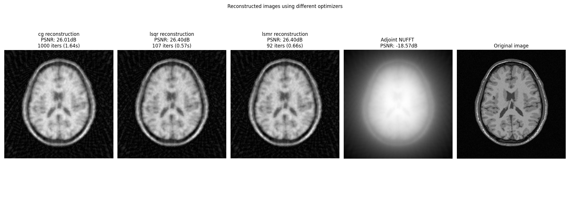
Display images#
fig, axs = plt.subplots(1, len(OPTIM) + 2, figsize=(20, 7))

for i, optim in enumerate(OPTIM):
    axs[i].imshow(abs(images[optim]), cmap="gray", origin="lower")
    axs[i].axis("off")
    axs[i].set_title(
        f"{optim} reconstruction\n PSNR: {iterations_cb[optim]['psnr'][-1]:.2f}dB \n"
        f"{len(iterations_cb[optim]['time'])} iters ({iterations_cb[optim]['time'][-1]:.2f}s)"
    )

axs[-1].imshow(abs(ground_truth), cmap="gray", origin="lower")
axs[-1].axis("off")
axs[-1].set_title("Original image")
axs[-2].imshow(
    abs(adjoint),
    cmap="gray",
    origin="lower",
)
axs[-2].axis("off")
axs[-2].set_title(
    f"Adjoint NUFFT \n PSNR: {psnr(abs(adjoint), abs(ground_truth), data_range=ground_truth.max()):.2f}dB"
)

fig.suptitle("Reconstructed images using different optimizers")
fig.tight_layout()
plt.show()
Total running time of the script: (0 minutes 33.668 seconds)