Trajectory constraints

A collection of methods to make trajectories fit hardware constraints.

Hereafter we illustrate different methods to reduce the gradient strengths and slew rates required for the trajectory to match the hardware constraints of MRI machines. A summary table is available below.

# Internal
import mrinufft as mn
from mrinufft.trajectories.utils import Acquisition, compute_gradients_and_slew_rates
from utils import show_trajectory_full

# External
import numpy as np

Script options

These options are used in the examples below as default values for all trajectories.

# Acquisition parameters
acq = Acquisition.default

# Trajectory parameters
Nc = 4  # Number of shots
Ns = 512  # Number of samples per shot
in_out = False  # Choose between in-out or center-out trajectories
nb_revolutions = 4  # Number of zigzags for base trajectories

# Display parameters
figure_size = 10  # Figure size for trajectory plots
subfigure_size = 6  # Figure size for subplots
one_shot = 2 * Nc // 3  # Highlight one shot in particular
sample_freq = 60  # Frequency of samples to display in the trajectory plots

We will be using a cone trajectory to showcase the different methods as it switches several times between high gradients and slew rates.

original_trajectory = mn.initialize_2D_spiral(
    Nc, Ns, in_out=in_out, nb_revolutions=nb_revolutions
)

show_trajectory_full(
    original_trajectory, one_shot, subfigure_size, sample_freq, acq=acq
)

grads, slews = compute_gradients_and_slew_rates(original_trajectory, acq)
grad_max, slew_max = np.max(grads), np.max(slews)
print(f"Max gradient: {grad_max:.3f} T/m, Max slew rate: {slew_max:.3f} T/m/ms")

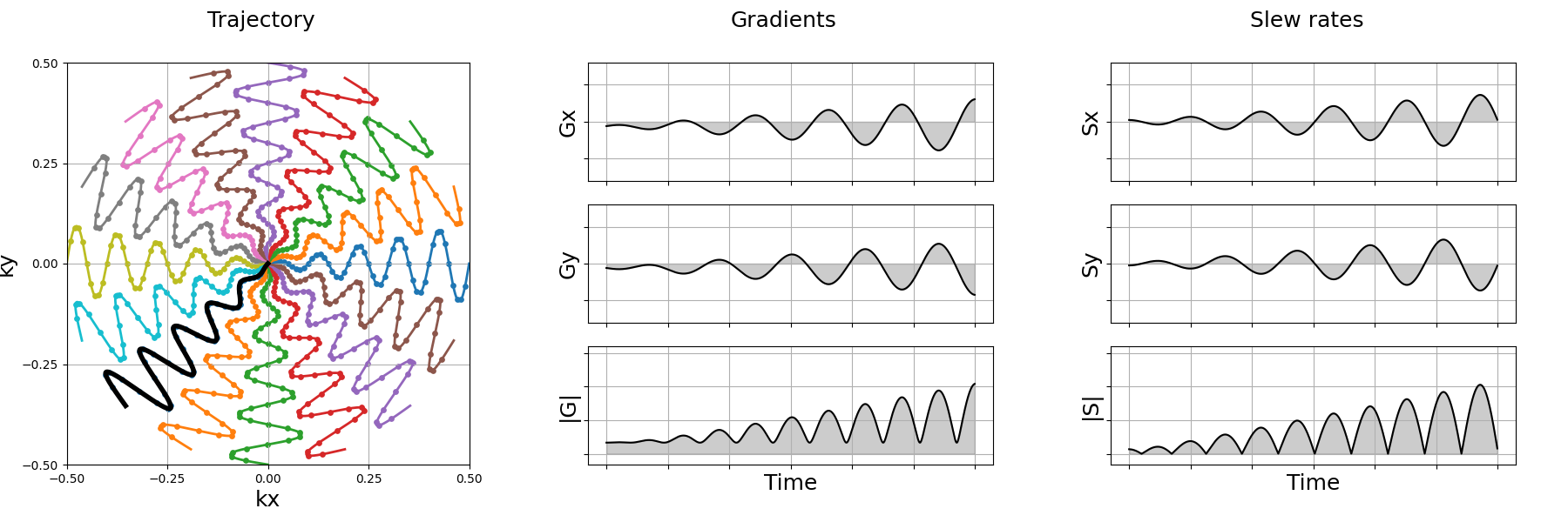
Max gradient: 0.058 T/m, Max slew rate: 282.015 T/m/ms

Arc-length parameterization

Arc-length parameterization is the simplest method to reduce the gradient strength as it resamples the trajectory to have a constant distance between samples. This is technically the lowest gradient strength achievable while preserving the path of the trajectory, but it does not preserve the k-space density and can lead to high slew rates as shown below.

from mrinufft.trajectories.projection import parameterize_by_arc_length

projected_trajectory = parameterize_by_arc_length(original_trajectory)

show_trajectory_full(
    projected_trajectory, one_shot, subfigure_size, sample_freq, acq=acq
)

grads, slews = compute_gradients_and_slew_rates(projected_trajectory, acq)
grad_max, slew_max = np.max(grads), np.max(slews)
print(f"Max gradient: {grad_max:.3f} T/m, Max slew rate: {slew_max:.3f} T/m/ms")

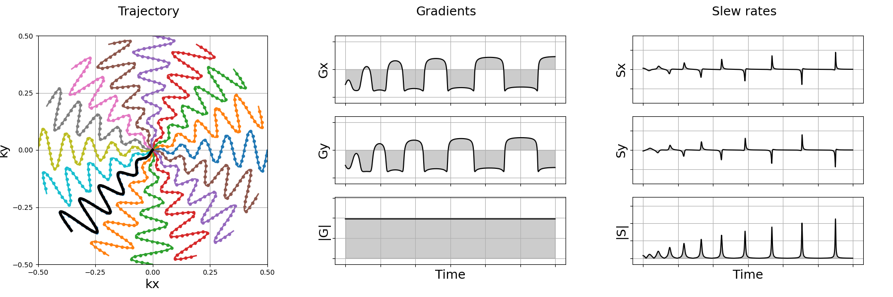
Max gradient: 0.029 T/m, Max slew rate: 2382.048 T/m/ms

Projection onto convex sets

The projection step is a primal-dual algorithm to project any trajectory into the convex constraint set. This step guarantees that the final trajectory is playably by the scanner. Also, as the constraint set if convex, the projection results in unique trajectory which is closest to the original one while being hardware compliant.

from mrinufft.trajectories.projection import project_trajectory

projected_trajectory = project_trajectory(
    original_trajectory,
    acq,
    max_iter=10000,
    TE_pos=0,
)

  0%|          | 0/10000 [00:00<?, ?it/s]
  1%|          | 121/10000 [00:00<00:08, 1200.73it/s]
  2%|▏         | 242/10000 [00:00<00:08, 1205.89it/s]
  4%|▎         | 363/10000 [00:00<00:07, 1206.89it/s]
  5%|▍         | 489/10000 [00:00<00:07, 1226.16it/s]
  6%|▌         | 612/10000 [00:00<00:07, 1222.50it/s]
  7%|▋         | 741/10000 [00:00<00:07, 1244.87it/s]
  9%|▊         | 870/10000 [00:00<00:07, 1259.28it/s]
 10%|▉         | 999/10000 [00:00<00:07, 1266.41it/s]
 11%|█▏        | 1129/10000 [00:00<00:06, 1275.05it/s]
 13%|█▎        | 1259/10000 [00:01<00:06, 1282.29it/s]
 14%|█▍        | 1389/10000 [00:01<00:06, 1285.61it/s]
 15%|█▌        | 1519/10000 [00:01<00:06, 1289.41it/s]
 16%|█▋        | 1650/10000 [00:01<00:06, 1293.18it/s]
 18%|█▊        | 1780/10000 [00:01<00:06, 1284.20it/s]
 19%|█▉        | 1909/10000 [00:01<00:06, 1266.58it/s]
 20%|██        | 2036/10000 [00:01<00:06, 1258.48it/s]
 22%|██▏       | 2167/10000 [00:01<00:06, 1272.25it/s]
 23%|██▎       | 2296/10000 [00:01<00:06, 1277.20it/s]
 24%|██▍       | 2426/10000 [00:01<00:05, 1282.86it/s]
 26%|██▌       | 2555/10000 [00:02<00:05, 1283.22it/s]
 27%|██▋       | 2685/10000 [00:02<00:05, 1287.72it/s]
 28%|██▊       | 2816/10000 [00:02<00:05, 1293.72it/s]
 29%|██▉       | 2946/10000 [00:02<00:05, 1293.79it/s]
 31%|███       | 3077/10000 [00:02<00:05, 1296.88it/s]
 32%|███▏      | 3207/10000 [00:02<00:05, 1291.02it/s]
 33%|███▎      | 3338/10000 [00:02<00:05, 1294.94it/s]
 35%|███▍      | 3468/10000 [00:02<00:05, 1292.54it/s]
 36%|███▌      | 3598/10000 [00:02<00:04, 1294.39it/s]
 37%|███▋      | 3728/10000 [00:02<00:04, 1292.01it/s]
 39%|███▊      | 3858/10000 [00:03<00:04, 1293.39it/s]
 40%|███▉      | 3989/10000 [00:03<00:04, 1296.66it/s]
 41%|████      | 4119/10000 [00:03<00:04, 1293.93it/s]
 42%|████▎     | 4250/10000 [00:03<00:04, 1296.18it/s]
 44%|████▍     | 4381/10000 [00:03<00:04, 1298.53it/s]
 45%|████▌     | 4511/10000 [00:03<00:04, 1267.37it/s]
 46%|████▋     | 4642/10000 [00:03<00:04, 1278.21it/s]
 48%|████▊     | 4773/10000 [00:03<00:04, 1286.61it/s]
 49%|████▉     | 4903/10000 [00:03<00:03, 1288.00it/s]
 50%|█████     | 5032/10000 [00:03<00:03, 1287.78it/s]
 52%|█████▏    | 5161/10000 [00:04<00:03, 1284.70it/s]
 53%|█████▎    | 5291/10000 [00:04<00:03, 1289.24it/s]
 54%|█████▍    | 5422/10000 [00:04<00:03, 1292.90it/s]
 56%|█████▌    | 5553/10000 [00:04<00:03, 1293.27it/s]
 57%|█████▋    | 5683/10000 [00:04<00:03, 1287.00it/s]
 58%|█████▊    | 5813/10000 [00:04<00:03, 1290.26it/s]
 59%|█████▉    | 5944/10000 [00:04<00:03, 1294.59it/s]
 61%|██████    | 6075/10000 [00:04<00:03, 1296.85it/s]
 62%|██████▏   | 6205/10000 [00:04<00:02, 1293.09it/s]
 63%|██████▎   | 6335/10000 [00:04<00:02, 1292.75it/s]
 65%|██████▍   | 6465/10000 [00:05<00:02, 1294.90it/s]
 66%|██████▌   | 6595/10000 [00:05<00:02, 1294.00it/s]
 67%|██████▋   | 6725/10000 [00:05<00:02, 1294.94it/s]
 69%|██████▊   | 6855/10000 [00:05<00:02, 1295.53it/s]
 70%|██████▉   | 6985/10000 [00:05<00:02, 1293.36it/s]
 71%|███████   | 7115/10000 [00:05<00:02, 1275.03it/s]
 72%|███████▏  | 7243/10000 [00:05<00:02, 1258.95it/s]
 74%|███████▎  | 7369/10000 [00:05<00:02, 1251.48it/s]
 75%|███████▍  | 7495/10000 [00:05<00:02, 1246.78it/s]
 76%|███████▌  | 7620/10000 [00:05<00:01, 1242.72it/s]
 77%|███████▋  | 7745/10000 [00:06<00:01, 1237.04it/s]
 79%|███████▊  | 7869/10000 [00:06<00:01, 1236.40it/s]
 80%|███████▉  | 7993/10000 [00:06<00:01, 1234.52it/s]
 81%|████████  | 8117/10000 [00:06<00:01, 1233.77it/s]
 82%|████████▏ | 8241/10000 [00:06<00:01, 1231.39it/s]
 84%|████████▎ | 8365/10000 [00:06<00:01, 1229.91it/s]
 85%|████████▍ | 8488/10000 [00:06<00:01, 1228.51it/s]
 86%|████████▌ | 8611/10000 [00:06<00:01, 1228.47it/s]
 87%|████████▋ | 8735/10000 [00:06<00:01, 1229.69it/s]
 89%|████████▊ | 8858/10000 [00:06<00:00, 1229.74it/s]
 90%|████████▉ | 8982/10000 [00:07<00:00, 1231.27it/s]
 91%|█████████ | 9106/10000 [00:07<00:00, 1229.58it/s]
 92%|█████████▏| 9229/10000 [00:07<00:00, 1227.58it/s]
 94%|█████████▎| 9352/10000 [00:07<00:00, 1227.88it/s]
 95%|█████████▍| 9476/10000 [00:07<00:00, 1229.94it/s]
 96%|█████████▌| 9600/10000 [00:07<00:00, 1230.64it/s]
 97%|█████████▋| 9724/10000 [00:07<00:00, 1231.95it/s]
 98%|█████████▊| 9848/10000 [00:07<00:00, 1232.26it/s]
100%|█████████▉| 9972/10000 [00:07<00:00, 1231.90it/s]
100%|██████████| 10000/10000 [00:07<00:00, 1266.42it/s]

show_trajectory_full(
    projected_trajectory, one_shot, subfigure_size, sample_freq, acq=acq
)
grads, slews = compute_gradients_and_slew_rates(projected_trajectory, acq)
grad_max, slew_max = np.max(grads), np.max(slews)
print(f"Max gradient: {grad_max:.3f} T/m, Max slew rate: {slew_max:.3f} T/m/ms")

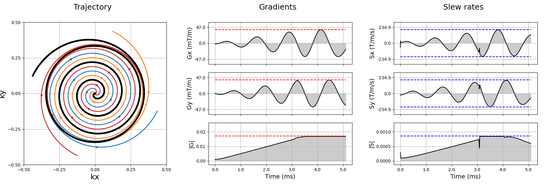
Max gradient: 0.040 T/m, Max slew rate: 197.972 T/m/ms