Gridded trajectory display

In this example, we show some tools available to display 3D trajectories. It can be used to understand the k-space sampling patterns, visualize the trajectories, see the sampling times, gradient strengths, slew rates etc. Another key feature is to display the sampling density in k-space, for example to check for k-space holes or irregularities in the learning-based trajectories that would lead to artifacts in the images.

# Imports
from mrinufft.trajectories.display3D import get_gridded_trajectory
import mrinufft.trajectories.trajectory3D as mtt
from mrinufft.trajectories.utils import Gammas
import matplotlib.pyplot as plt
import numpy as np

Helper function to Displaying 3D Gridded Trajectories

Utility function to plot mid-plane slices for 3D volumes

def plot_slices(axs, volume, title=""):
    def set_labels(ax, axis_num=None):
        ax.set_xticks([0, 32, 64])
        ax.set_yticks([0, 32, 64])
        ax.set_xticklabels([r"$-\pi$", 0, r"$\pi$"])
        ax.set_yticklabels([r"$-\pi$", 0, r"$\pi$"])
        if axis_num is not None:
            ax.set_xlabel(r"$k_" + "zxy"[axis_num] + r"$")
            ax.set_ylabel(r"$k_" + "yzx"[axis_num] + r"$")

    for i in range(3):
        volume = np.rollaxis(volume, i, 0)
        axs[i].imshow(volume[volume.shape[0] // 2])
        axs[i].set_title(
            ((title + f"\n") if i == 0 else "") + r"$k_{" + "xyz"[i] + r"}=0$"
        )
        set_labels(axs[i], i)

Helper function to Displaying 3D Trajectories

Helper function to showcase the features of get_gridded_trajectory function This function will first grid the trajectory using the get_gridded_trajectory function and then plot the mid-plane slices of the gridded trajectory.

def create_grid(grid_type, trajectories, traj_params, **kwargs):
    fig, axs = plt.subplots(3, 3, figsize=(10, 10))
    plt.subplots_adjust(hspace=0.5)
    for i, (name, traj) in enumerate(trajectories.items()):
        grid = get_gridded_trajectory(
            traj,
            traj_params["img_size"],
            grid_type=grid_type,
            traj_params=traj_params,
            **kwargs,
        )
        plot_slices(axs[:, i], grid, title=name)

Trajectories to display

We instantiate a bunch of sampling trajectories to display hereafter with get_gridded_trajectory and previous helper functions.

trajectories = {
    "Radial": mtt.initialize_3D_phyllotaxis_radial(64 * 8, 64),
    "FLORET": mtt.initialize_3D_floret(64 * 8, 64, nb_revolutions=2),
    "Seiffert Spirals": mtt.initialize_3D_seiffert_spiral(64 * 8, 64),
}
traj_params = {
    "FOV": (0.23, 0.23, 0.23),
    "img_size": (64, 64, 64),
    "gamma": Gammas.HYDROGEN,
}

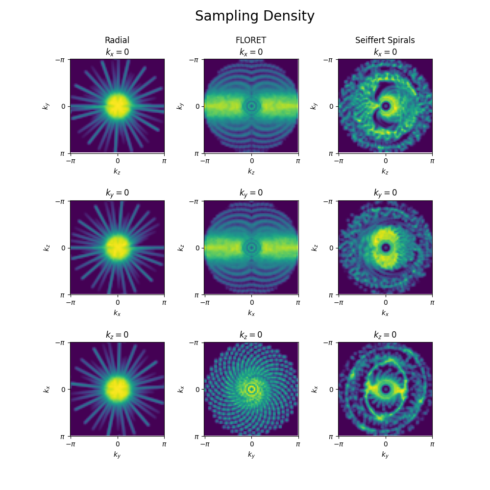
Sampling density

Display the density of the trajectories, along the 3 mid-planes. For this, make grid_type=”density”.

create_grid("density", trajectories, traj_params)
plt.suptitle("Sampling Density", y=0.98, x=0.52, fontsize=20)
plt.show()

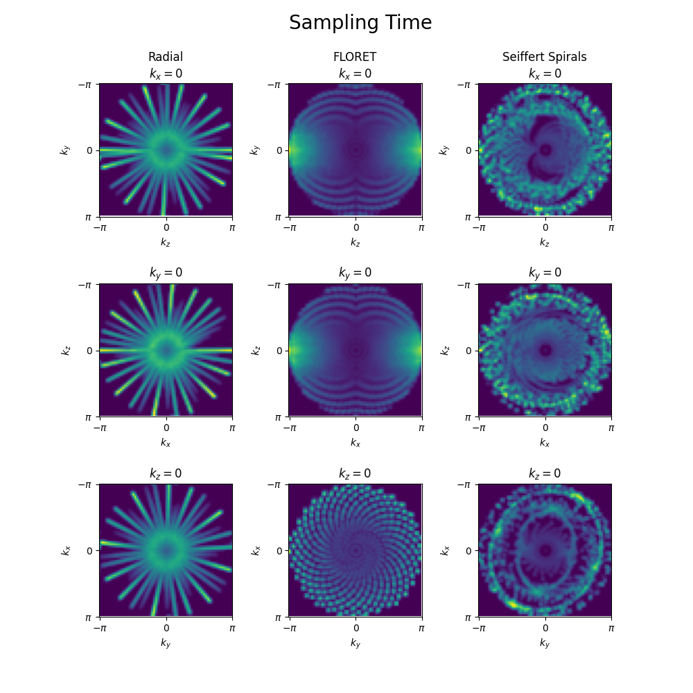
Sampling time

Display the sampling times over the trajectories. For this, make grid_type=”time”. It helps to check the sampling times over the k-space trajectories, which can be responsible for excessive off-resonance artifacts. Note that this is just a relative visualization of sample times on a colour scale, and the actual sampling time.

create_grid("time", trajectories, traj_params)
plt.suptitle("Sampling Time", y=0.98, x=0.52, fontsize=20)
plt.show()

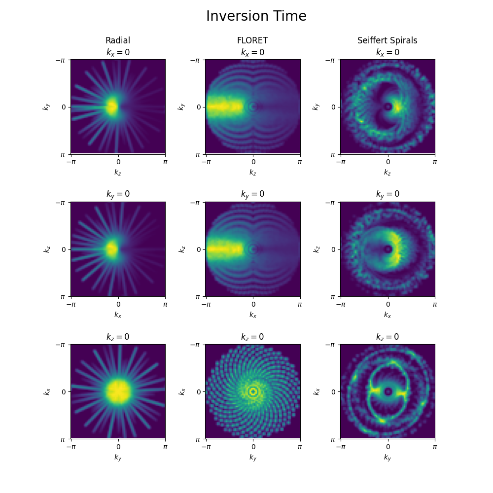
Inversion time

Display the inversion time of the trajectories. For this, make grid_type=”inversion”. This helps in obtaining the inversion time when particular region of k-space is sampled, assuming the trajectories are time ordered, and the argument turbo_factor is specified, which is the time between 2 inversion pulses.

create_grid("inversion", trajectories, traj_params, turbo_factor=64)
plt.suptitle("Inversion Time", y=0.98, x=0.52, fontsize=20)
plt.show()

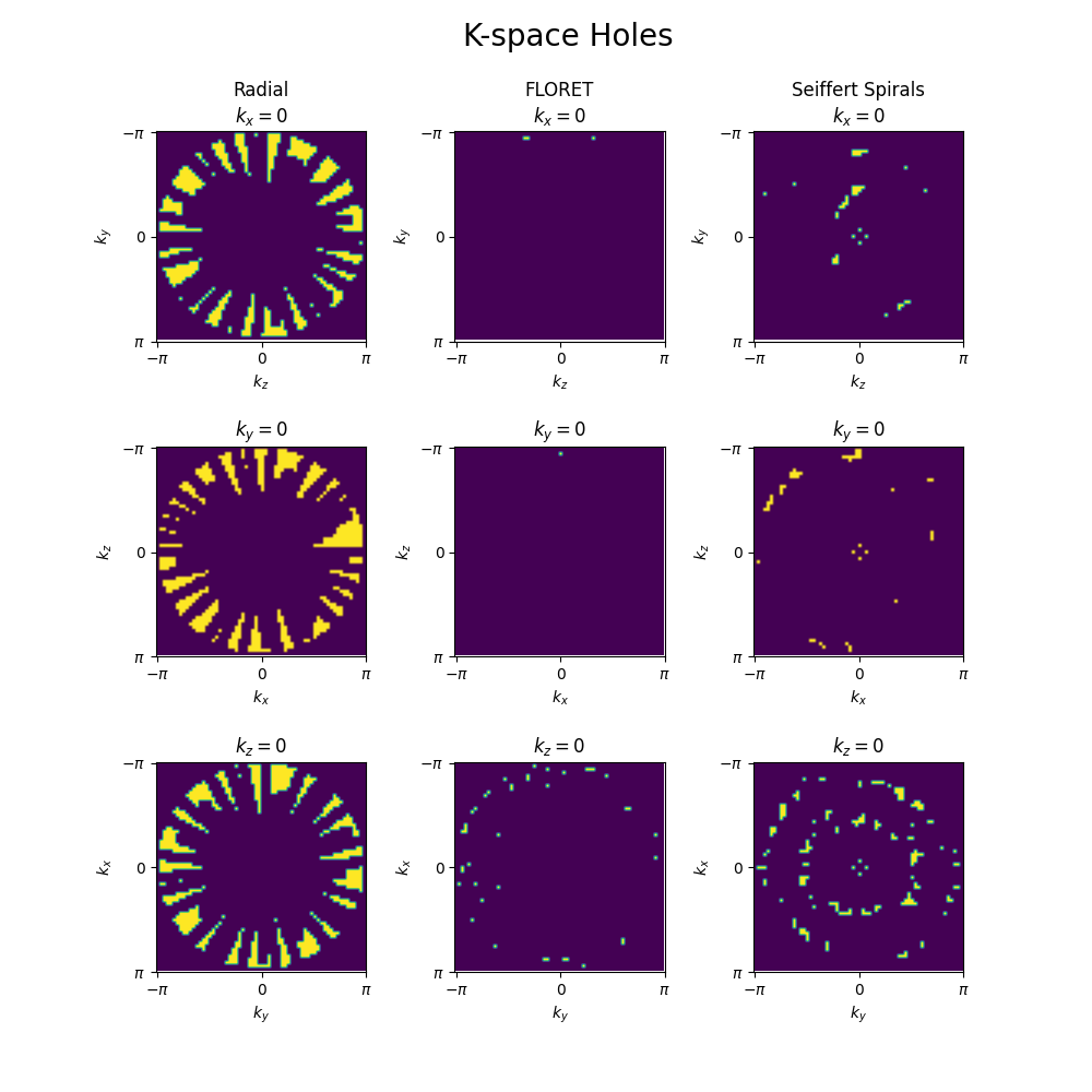
K-space holes

Display the k-space holes in the trajectories. For this, make grid_type=”holes”. K-space holes are areas with missing trajectory coverage, and can typically occur with learning-based trajectories when optimized using a specific loss. This feature can be used to identify the k-space holes, which could lead to Gibbs-like ringing artifacts in the images.

create_grid("holes", trajectories, traj_params, threshold=1e-2)
plt.suptitle("K-space Holes", y=0.98, x=0.52, fontsize=20)
plt.show()

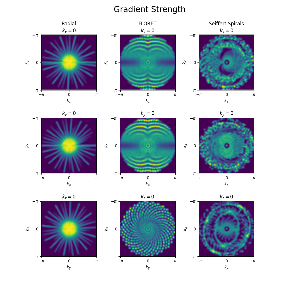
Gradient strength

Display the gradient strength of the trajectories. For this, make grid_type=”gradients”. This helps in displaying the gradient strength applied at specific k-space region, which can be used as a surrogate to k-space “velocity”, i.e. how fast does trajectory pass through a given region in k-space. It could be useful while characterizing spatial SNR profile in k-space

create_grid("gradients", trajectories, traj_params)
plt.suptitle("Gradient Strength", y=0.98, x=0.52, fontsize=20)
plt.show()

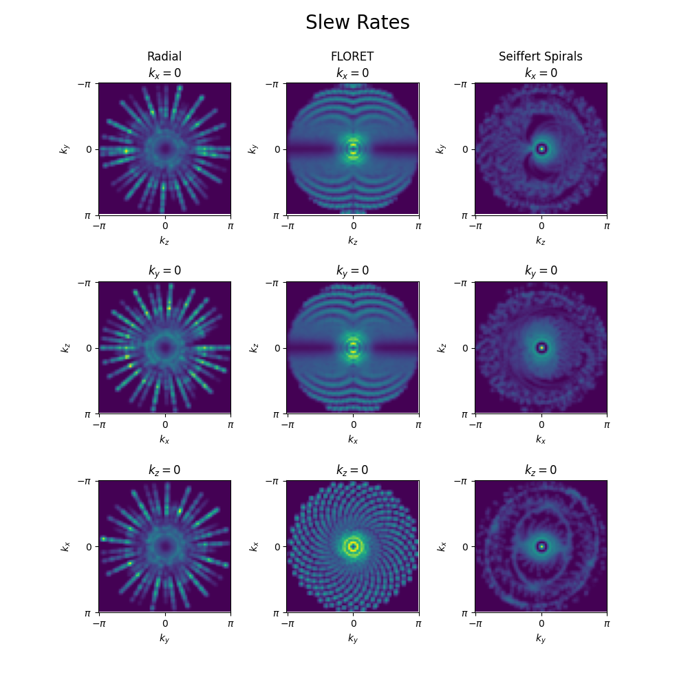
Slew rates

Display the slew rates of the trajectories. For this, make grid_type=”slew”. This helps in displaying the slew rates applied at specific k-space region, which can ne used as a surrogate to k-space “acceleration”, i.e. how fast does trajectory change in a given region in k-space It could be useful to understand potential regions in k-space with eddy current artifacts and trajectories which could lead to peripheral nerve stimulations.

create_grid("slew", trajectories, traj_params)
plt.suptitle("Slew Rates", y=0.98, x=0.52, fontsize=20)
plt.show()