
Note
Go to the end to download the full example code or to run this example in your browser via Binder.
Sensitivity maps estimation#
This example demonstrates how to estimate coil sensitivity maps from
non-Cartesian k-space data using different methods provided in the
mrinufft.extras module.
We will simulate k-space data from a known MRI image and coil sensitivity
maps, and then estimate the sensitivity maps using the ESPIRiT method [espirit],
the PISCO method [pisco], and a low-frequency calibration method [sense].
We will visualize the estimated sensitivity maps and compare them to the
actual sensitivity maps used in the simulation.
Imports#
import matplotlib.pyplot as plt
import numpy as np
from brainweb_dl import get_mri
from sigpy.mri.sim import birdcage_maps

from mrinufft import get_operator
from mrinufft.extras import get_smaps
from mrinufft.trajectories import initialize_3D_floret
import cupy as cp
import os
Function to display imgs
def show_maps(imgs):
    """Display 4D sensitivity maps in a 4x3 figure layout."""
    n_coils, nx, ny, nz = imgs.shape
    fig, axes = plt.subplots(4, 3, figsize=(15, 20))
    imgs = np.abs(imgs)
    for i in range(n_coils):
        axes[i, 0].imshow(imgs[i, nx // 2, :, :], vmax=imgs.max(), vmin=imgs.min())
        axes[i, 1].imshow(imgs[i, :, ny // 2, :], vmax=imgs.max(), vmin=imgs.min())
        axes[i, 2].imshow(imgs[i, :, :, nz // 2], vmax=imgs.max(), vmin=imgs.min())
        axes[i, 0].set_title(f"Coil {i+1} - YZ plane")
        axes[i, 1].set_title(f"Coil {i+1} - XZ plane")
        axes[i, 2].set_title(f"Coil {i+1} - XY plane")
    plt.show()
    return fig


BACKEND = os.environ.get("MRINUFFT_BACKEND", "cufinufft")
Get MRI data, 3D FLORET trajectory, and simulate k-space data
samples_loc = initialize_3D_floret(Nc=16 * 16, Ns=256)
mri = get_mri(0)[::2, ::2, ::2][::-1, ::-1]  # Load and downsample MRI data for speed
n_coils = 4
actual_smaps = birdcage_maps(
    (n_coils, *mri.shape), dtype=np.complex64
)  # Generate birdcage sensitivity maps
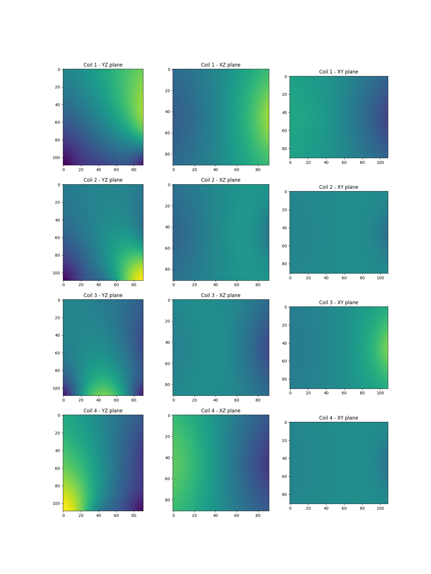
Show the sensitivity maps
show_maps(actual_smaps)
<Figure size 1500x2000 with 12 Axes>
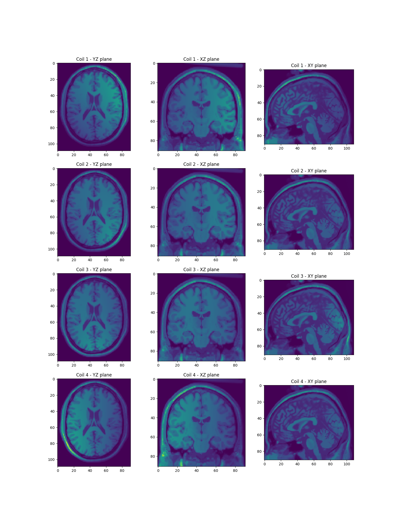
Show the per channel images
per_ch_mri = mri[None, ...] * actual_smaps  # Generate per-coil MRI data
show_maps(per_ch_mri)
<Figure size 1500x2000 with 12 Axes>
Simulate k-space data
forward_op = get_operator(BACKEND)(
    samples_loc, shape=mri.shape, n_coils=n_coils, density=True
)
kspace_data = forward_op.op(per_ch_mri)  # Simulate k-space data

if str.lower(BACKEND) in ["gpunufft", "cufinufft"]:
    # GPU exists, run on GPU
    import cupy as cp

    kspace_data = cp.asarray(kspace_data, dtype=cp.complex64)
    samples_loc = cp.asarray(samples_loc, dtype=cp.float32)
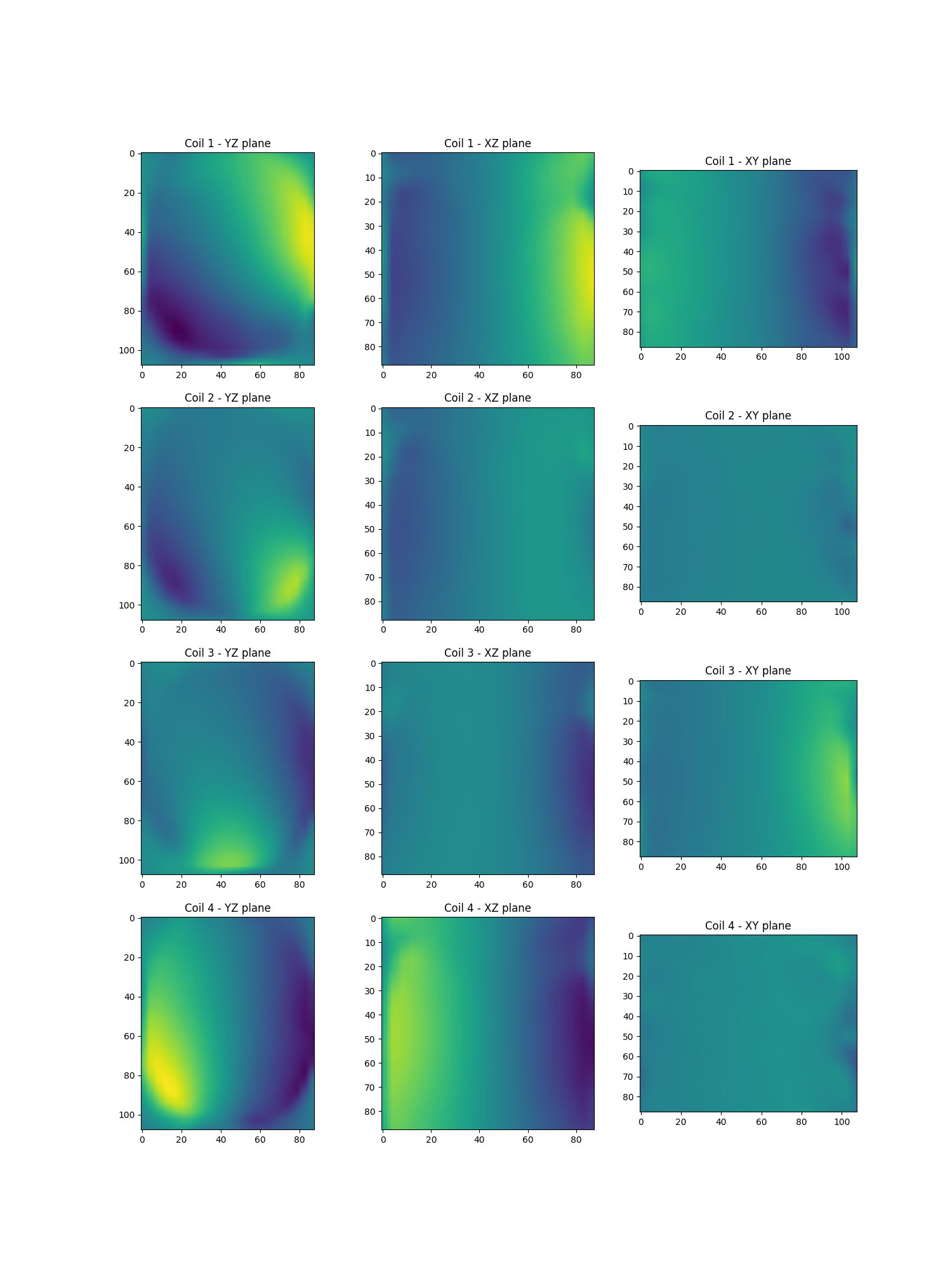
Estimate sensitivity maps using ESPIRiT
Smaps = get_smaps("espirit")(
    samples_loc,
    mri.shape,
    kspace_data=kspace_data,
    density=forward_op.density,
    backend=BACKEND,
    decim=4,
)
if str.lower(BACKEND) in ["gpunufft", "cufinufft"]:
    Smaps = Smaps.get()
show_maps(Smaps)
  0%|          | 0/10 [00:00<?, ?it/s]
 10%|█         | 1/10 [00:00<00:01,  8.26it/s]
 30%|███       | 3/10 [00:00<00:00, 11.19it/s]
 50%|█████     | 5/10 [00:00<00:00,  9.66it/s]
 70%|███████   | 7/10 [00:00<00:00, 10.77it/s]
 90%|█████████ | 9/10 [00:00<00:00, 11.41it/s]
100%|██████████| 10/10 [00:00<00:00, 10.93it/s]

<Figure size 1500x2000 with 12 Axes>
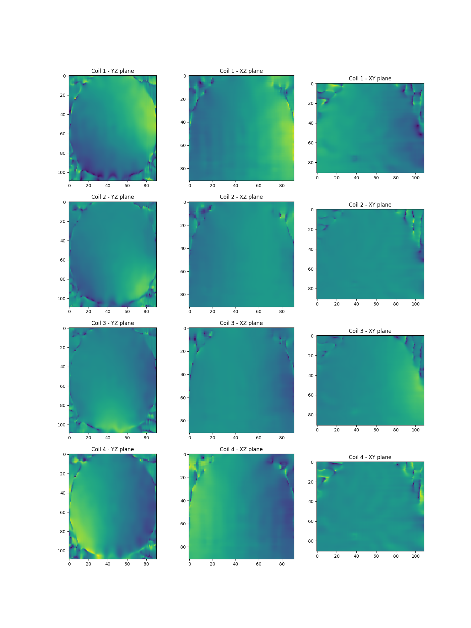
Estimate sensitivity maps using PISCO
Smaps = get_smaps("pisco")(
    samples_loc,
    mri.shape,
    kspace_data=kspace_data,
    density=forward_op.density,
    backend=BACKEND,
)
if str.lower(BACKEND) in ["gpunufft", "cufinufft"]:
    Smaps = Smaps.get()
show_maps(Smaps)
  0%|          | 0/10 [00:00<?, ?it/s]
 20%|██        | 2/10 [00:00<00:00, 12.97it/s]
 40%|████      | 4/10 [00:00<00:00, 12.96it/s]
 60%|██████    | 6/10 [00:00<00:00, 12.89it/s]
 80%|████████  | 8/10 [00:00<00:00, 12.84it/s]
100%|██████████| 10/10 [00:00<00:00, 12.77it/s]
100%|██████████| 10/10 [00:00<00:00, 12.81it/s]

<Figure size 1500x2000 with 12 Axes>
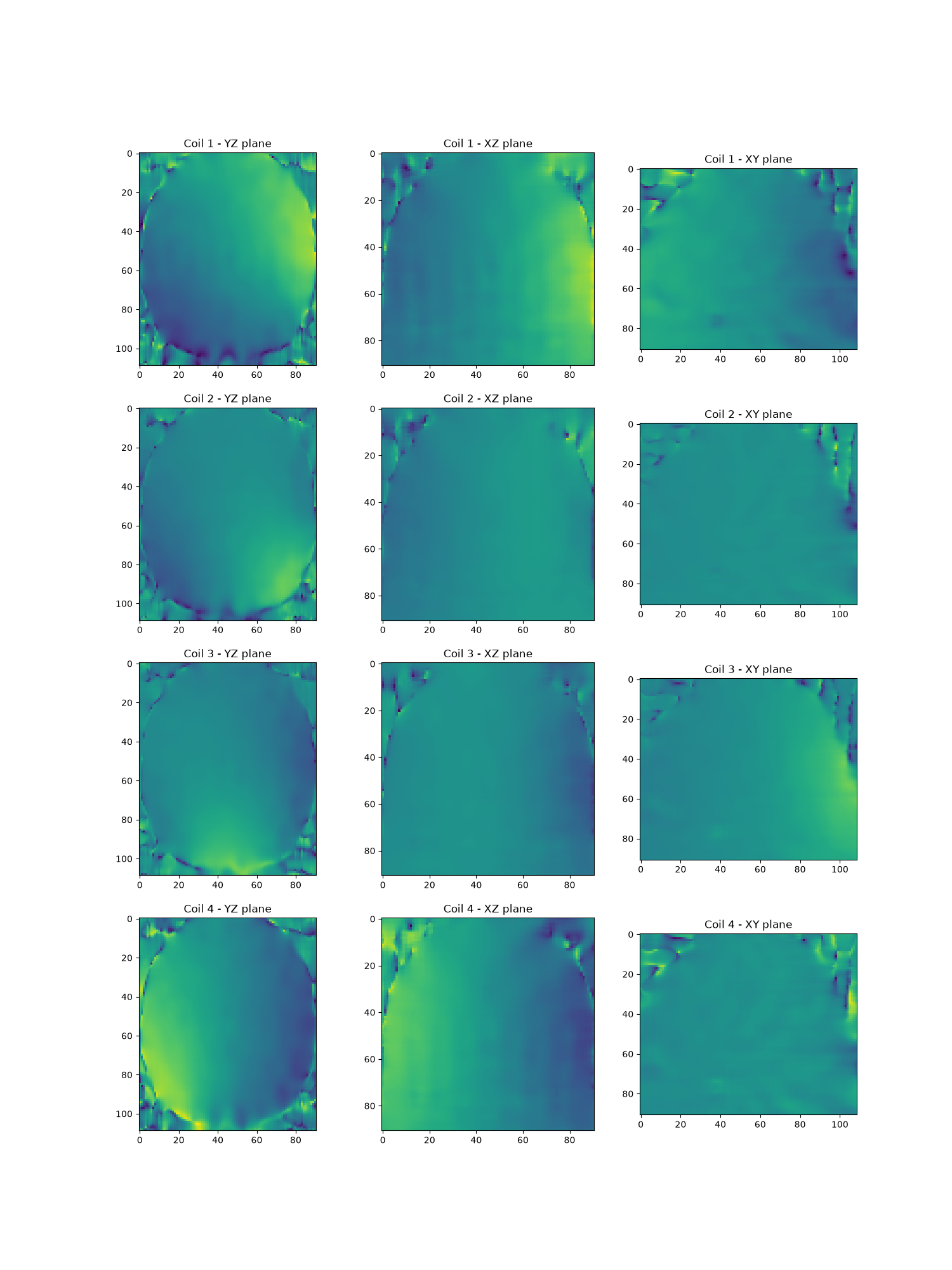
Estimate the sensitivity map using low-frequency calibration
Smaps = get_smaps("low_frequency")(
    samples_loc,
    mri.shape,
    kspace_data=kspace_data,
    density=forward_op.density,
    backend=BACKEND,
)

if str.lower(BACKEND) in ["gpunufft", "cufinufft"]:
    Smaps = Smaps.get()
show_maps(Smaps)
  0%|          | 0/10 [00:00<?, ?it/s]
 10%|█         | 1/10 [00:00<00:01,  8.60it/s]
 20%|██        | 2/10 [00:00<00:00,  8.60it/s]
 30%|███       | 3/10 [00:00<00:00,  8.34it/s]
 40%|████      | 4/10 [00:00<00:00,  7.96it/s]
 50%|█████     | 5/10 [00:00<00:00,  8.18it/s]
 60%|██████    | 6/10 [00:00<00:00,  8.32it/s]
 70%|███████   | 7/10 [00:00<00:00,  8.37it/s]
 80%|████████  | 8/10 [00:00<00:00,  8.06it/s]
 90%|█████████ | 9/10 [00:01<00:00,  8.22it/s]
100%|██████████| 10/10 [00:01<00:00,  8.38it/s]
100%|██████████| 10/10 [00:01<00:00,  8.29it/s]

<Figure size 1500x2000 with 12 Axes>
References#
Loubna El Gueddari, C. Lazarus, H Carrié, A. Vignaud, Philippe Ciuciu. Self-calibrating nonlinear reconstruction algorithms for variable density sampling and parallel reception MRI. 10th IEEE Sensor Array and Multichannel Signal Processing workshop, Jul 2018, Sheffield, United Kingdom. ⟨hal-01782428v1⟩
Uecker M, Lai P, Murphy MJ, Virtue P, Elad M, Pauly JM, Vasanawala SS, Lustig M. ESPIRiT–an eigenvalue approach to autocalibrating parallel MRI: where SENSE meets GRAPPA. Magn Reson Med. 2014 Mar;71(3):990-1001. doi: 10.1002/mrm.24751. PMID: 23649942; PMCID: PMC4142121.
R. A. Lobos, C.-C. Chan, J. P. Haldar. New Theory and Faster Computations for Subspace-Based Sensitivity Map Estimation in Multichannel MRI. IEEE Transactions on Medical Imaging 43:286-296, 2024. doi: 10.1109/TMI.2023.3299599.
Total running time of the script: (0 minutes 9.759 seconds)

