display_3D_trajectory#
- mrinufft.trajectories.display.display_3D_trajectory(trajectory: ndarray[tuple[int, ...], dtype[_ScalarType_co]], nb_repetitions: int | None = None, figsize: float = 5, per_plane: bool = True, one_shot: bool | int = False, subfigure: Figure | Axes | None = None, show_constraints: bool = False, acq: Acquisition | None = None, constraints_order: int | str | None = None) Axes[source]#
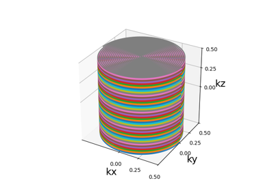
Display 3D trajectories.
- Parameters:
trajectory (NDArray) – Trajectory to display.
nb_repetitions (int) – Number of repetitions (planes, cones, shells, etc). The default is None.
figsize (float, optional) – Size of the figure.
per_plane (bool, optional) – If True, display the trajectory with a different color for each plane.
one_shot (bool or int, optional) – State if a specific shot should be highlighted in bold black. If True, highlight the middle shot. If int, highlight the shot at that index. The default is False.
subfigure (plt.Figure, plt.SubFigure or plt.Axes, optional) – The figure where the trajectory should be displayed. The default is None.
show_constraints (bool, optional) – Display the points where the gradients and slew rates are above the gmax and smax limits, respectively. The default is False.
acq (Acquisition, optional) – Acquisition configuration to use. If None, the default acquisition is used.
constraint_order (int, str, optional) – Norm order defining how the constraints are checked, typically 2 or np.inf, following the numpy.linalg.norm conventions on parameter ord. The default is None.
**kwargs – Acquisition parameters used to check on hardware constraints, following the parameter convention from mrinufft.trajectories.utils.compute_gradients_and_slew_rates.
- Returns:
ax – Axes of the figure.
- Return type:
plt.Axes