Reconstruction with conjugate gradient

An example to show how to reconstruct volumes using conjugate gradient method.

This script demonstrates the use of the Conjugate Gradient (CG) method for solving systems of linear equations of the form Ax = b, where A is a symmetric positive-definite matrix. The CG method is an iterative algorithm that is particularly useful for large, sparse systems where direct methods are computationally expensive.

The Conjugate Gradient method is widely used in various scientific and engineering applications, including solving partial differential equations, optimization problems, and machine learning tasks.

This method is inspired by techniques from [SigPy] and [Aquaulb] MOOC, as well as general knowledge in [Wikipedia].

Imports

import numpy as np
import mrinufft
from brainweb_dl import get_mri
from mrinufft.density import voronoi
from matplotlib import pyplot as plt

Setup Inputs

samples_loc = mrinufft.initialize_2D_spiral(Nc=64, Ns=512, nb_revolutions=8)
image = get_mri(sub_id=4)
image = np.flipud(image[90])

Setup the NUFFT operator

NufftOperator = mrinufft.get_operator("gpunufft")  # get the operator

nufft = NufftOperator(
    samples_loc,
    shape=image.shape,
    density=True,
)  # create the NUFFT operator

Reconstruct the image using the CG method

kspace_data = nufft.op(image)  # get the k-space data
dc_adjoint = nufft.adj_op(kspace_data)
reconstructed_image, loss = nufft.cg(
    kspace_data=kspace_data, x_init=dc_adjoint.copy(), num_iter=50, compute_loss=True
)


# Display the results

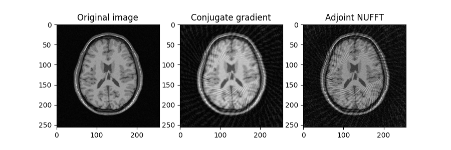
plt.figure(figsize=(15, 10))
plt.subplot(2, 3, 1)
plt.title("Original image")
plt.imshow(image, cmap="gray")
plt.colorbar()

plt.subplot(2, 3, 2)
plt.title("Conjugate gradient")
plt.imshow(abs(reconstructed_image), vmin=image.min(), vmax=image.max(), cmap="gray")
plt.colorbar()

plt.subplot(2, 3, 3)
plt.title("Adjoint NUFFT")
plt.imshow(
    abs(nufft.adj_op(kspace_data)), vmin=image.min(), vmax=image.max(), cmap="gray"
)
plt.colorbar()

plt.subplot(2, 3, 4)
plt.title("Loss")
plt.plot(loss)
plt.grid()

plt.subplot(2, 3, 5)
plt.title("K-space from conjugate gradient (CG)")
plt.plot(np.log(abs(kspace_data)), label="Acquired k-space")
plt.plot(np.log(abs(nufft.op(reconstructed_image))), label="CG k-space")
plt.legend(loc="lower left", fontsize=8)

plt.subplot(2, 3, 6)
plt.title("K-space from DC adjoint NUFFT")
plt.plot(np.log(abs(kspace_data)), label="Acquired k-space")
plt.plot(np.log(abs(nufft.op(dc_adjoint))), label="DC adjoint k-space")
plt.legend(loc="lower left", fontsize=8)

<matplotlib.legend.Legend object at 0x7b3a692c9150>

References

[SigPy]

SigPy Documentation. Conjugate Gradient Method. https://sigpy.readthedocs.io/en/latest/_modules/sigpy/alg.html#ConjugateGradient

[Aquaulb]

Aquaulb’s MOOC: Solving PDE with Iterative Methods. https://aquaulb.github.io/book_solving_pde_mooc/solving_pde_mooc/notebooks/05_IterativeMethods/05_02_Conjugate_Gradient.html

[Wikipedia]

Wikipedia: Conjugate Gradient Method. https://en.wikipedia.org/wiki/Conjugate_gradient_method