Density Compensation Routines

Examples of differents density compensation methods.

Density compensation depends on the sampling trajectory,and is apply before the adjoint operation to act as preconditioner, and should make the lipschitz constant of the operator roughly equal to 1.

import brainweb_dl as bwdl

import matplotlib.pyplot as plt
import numpy as np
from mrinufft import get_density, get_operator, check_backend
from mrinufft.trajectories import initialize_2D_radial
from mrinufft.trajectories.display import display_2D_trajectory

Create sample data

mri_2D = bwdl.get_mri(4, "T1")[80, ...].astype(np.float32)

print(mri_2D.shape)

traj = initialize_2D_radial(192, 192).astype(np.float32)

nufft = get_operator("finufft")(traj, mri_2D.shape, density=False)
kspace = nufft.op(mri_2D)
adjoint = nufft.adj_op(kspace)

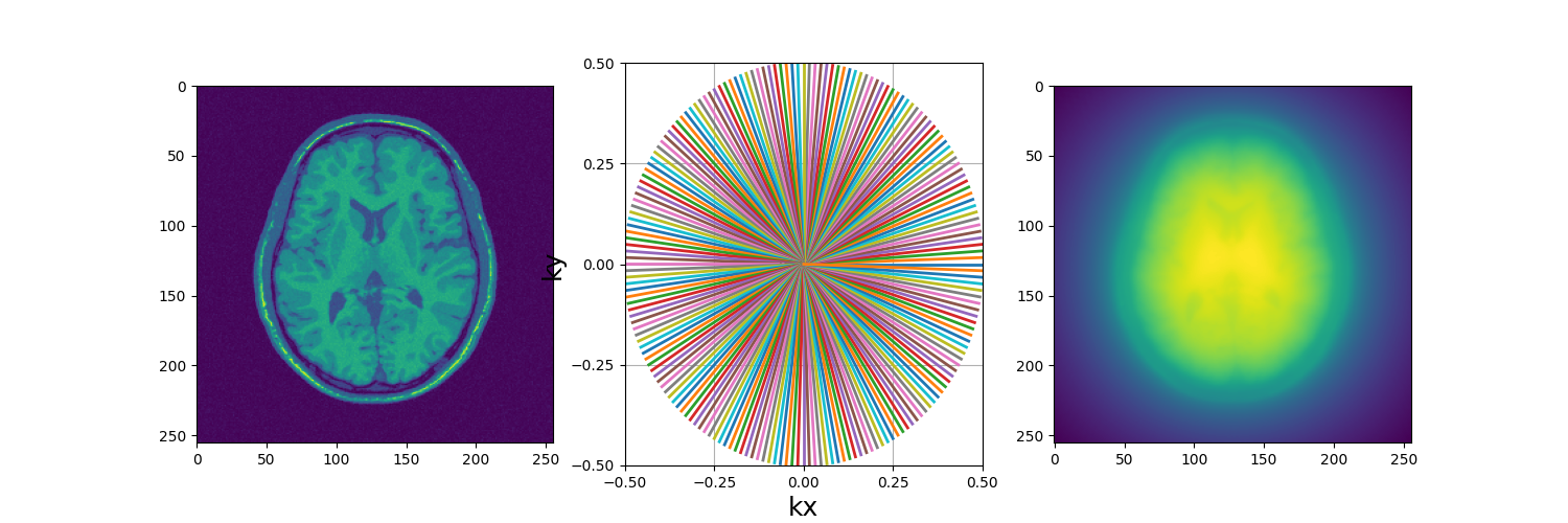
fig, axs = plt.subplots(1, 3, figsize=(15, 5))
axs[0].imshow(abs(mri_2D))
display_2D_trajectory(traj, subfigure=axs[1])
axs[2].imshow(abs(adjoint))

Downloading subject04_t1w: 0.00B [00:00, ?B/s]


Downloading subject04_t1w: 1.00kB [00:04, 209B/s]


Downloading subject04_t1w: 112kB [00:05, 32.4kB/s]


Downloading subject04_t1w: 261kB [00:05, 89.8kB/s]


Downloading subject04_t1w: 465kB [00:05, 193kB/s]


Downloading subject04_t1w: 721kB [00:05, 358kB/s]


Downloading subject04_t1w: 1.02MB [00:05, 612kB/s]


Downloading subject04_t1w: 1.42MB [00:05, 1.01MB/s]


Downloading subject04_t1w: 1.92MB [00:05, 1.57MB/s]


Downloading subject04_t1w: 2.57MB [00:05, 2.40MB/s]


Downloading subject04_t1w: 3.26MB [00:05, 3.29MB/s]


Downloading subject04_t1w: 3.99MB [00:05, 4.20MB/s]


Downloading subject04_t1w: 4.63MB [00:06, 4.78MB/s]


Downloading subject04_t1w: 5.29MB [00:06, 5.32MB/s]


Downloading subject04_t1w: 5.96MB [00:06, 5.77MB/s]


Downloading subject04_t1w: 6.59MB [00:06, 6.00MB/s]


Downloading subject04_t1w: 7.26MB [00:06, 6.26MB/s]


Downloading subject04_t1w: 7.90MB [00:06, 6.39MB/s]


Downloading subject04_t1w: 8.54MB [00:06, 6.41MB/s]


Downloading subject04_t1w: 9.20MB [00:06, 6.48MB/s]


Downloading subject04_t1w: 9.84MB [00:06, 6.50MB/s]


Downloading subject04_t1w: 10.5MB [00:06, 6.46MB/s]


Downloading subject04_t1w: 11.1MB [00:07, 6.31MB/s]


Downloading subject04_t1w: 11.7MB [00:07, 6.27MB/s]


Downloading subject04_t1w: 12.3MB [00:07, 6.12MB/s]


Downloading subject04_t1w: 12.9MB [00:07, 5.86MB/s]


Downloading subject04_t1w: 13.5MB [00:07, 5.67MB/s]


Downloading subject04_t1w: 14.0MB [00:07, 5.38MB/s]


Downloading subject04_t1w: 14.5MB [00:07, 5.09MB/s]


Downloading subject04_t1w: 15.0MB [00:07, 4.85MB/s]


Downloading subject04_t1w: 15.5MB [00:08, 4.63MB/s]


Downloading subject04_t1w: 15.9MB [00:08, 4.51MB/s]


                                                   (256, 256)
/opt/hostedtoolcache/Python/3.10.14/x64/lib/python3.10/site-packages/mrinufft/_utils.py:87: UserWarning: Samples will be rescaled to [-pi, pi), assuming they were in [-0.5, 0.5)
  warnings.warn(
/opt/hostedtoolcache/Python/3.10.14/x64/lib/python3.10/site-packages/finufft/_interfaces.py:329: UserWarning: Argument `data` does not satisfy the following requirement: C. Copying array (this may reduce performance)
  warnings.warn(f"Argument `{name}` does not satisfy the following requirement: {prop}. Copying array (this may reduce performance)")

<matplotlib.image.AxesImage object at 0x7fae491ca800>

As you can see, the radial sampling pattern as a strong concentration of sampling point in the center, resulting in a low-frequency biased adjoint reconstruction.

Geometry based methods

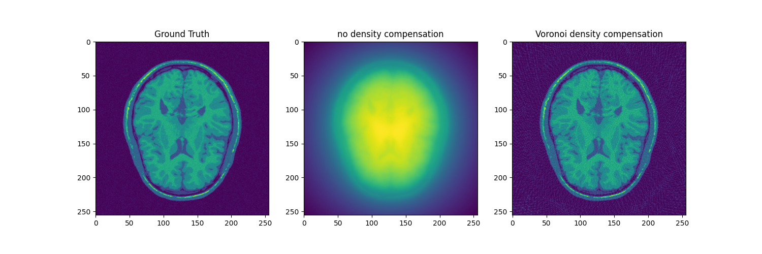
Voronoi

Voronoi Parcellation attribute a weights to each k-space coordinate, inversely proportional to its voronoi cell area.

# .. warning::
#    The current implementation of voronoi parcellation is CPU only, and is thus
#    **very** slow in 3D ( > 1h).

voronoi_weights = get_density("voronoi", traj)

nufft_voronoi = get_operator("finufft")(
    traj, shape=mri_2D.shape, density=voronoi_weights
)
adjoint_voronoi = nufft_voronoi.adj_op(kspace)
fig, axs = plt.subplots(1, 3, figsize=(15, 5))
axs[0].imshow(abs(mri_2D))
axs[0].set_title("Ground Truth")
axs[1].imshow(abs(adjoint))
axs[1].set_title("no density compensation")
axs[2].imshow(abs(adjoint_voronoi))
axs[2].set_title("Voronoi density compensation")

/opt/hostedtoolcache/Python/3.10.14/x64/lib/python3.10/site-packages/mrinufft/_utils.py:87: UserWarning: Samples will be rescaled to [-pi, pi), assuming they were in [-0.5, 0.5)
  warnings.warn(

Text(0.5, 1.0, 'Voronoi density compensation')

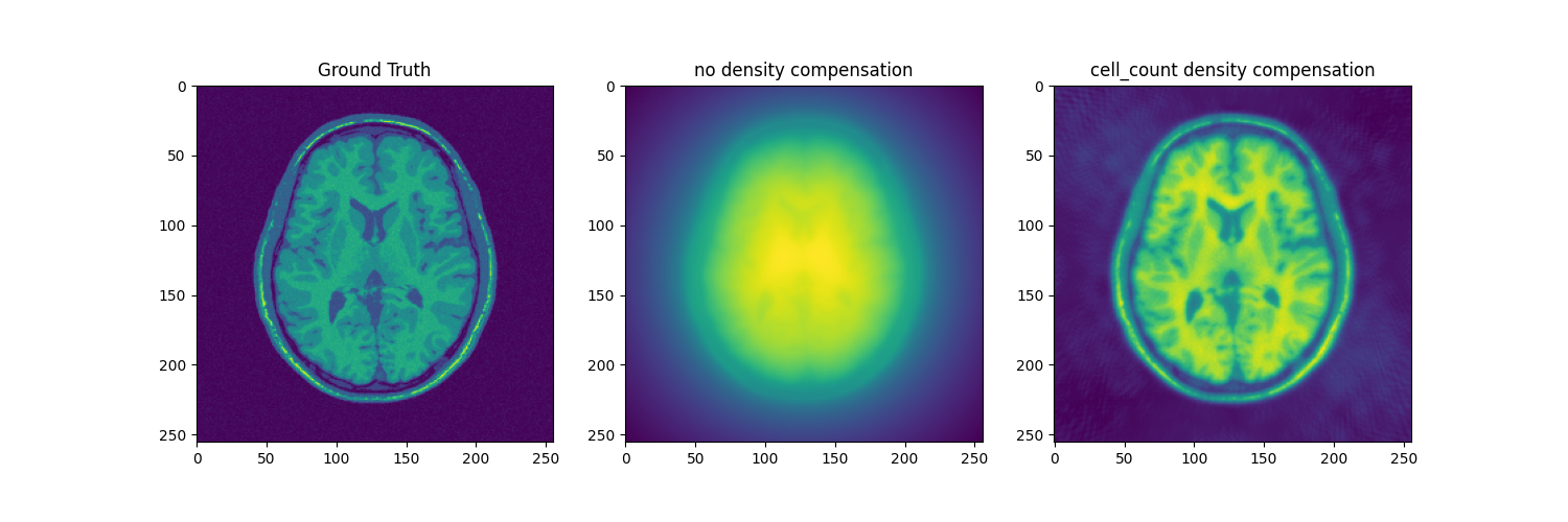
Cell Counting

Cell Counting attributes weights based on the number of trajectory point lying in a same k-space nyquist voxel. This can be viewed as an approximation to the voronoi neth

# .. note::
#    Cell counting is faster than voronoi (especially in 3D), but is less precise.

# The size of the niquist voxel can be tweak by using the osf parameter. Typically as the NUFFT (and by default in MRI-NUFFT) is performed at an OSF of 2

cell_count_weights = get_density("cell_count", traj, shape=mri_2D.shape, osf=2.0)

nufft_cell_count = get_operator("finufft")(
    traj, shape=mri_2D.shape, density=cell_count_weights, upsampfac=2.0
)
adjoint_cell_count = nufft_cell_count.adj_op(kspace)
fig, axs = plt.subplots(1, 3, figsize=(15, 5))
axs[0].imshow(abs(mri_2D))
axs[0].set_title("Ground Truth")
axs[1].imshow(abs(adjoint))
axs[1].set_title("no density compensation")
axs[2].imshow(abs(adjoint_cell_count))
axs[2].set_title("cell_count density compensation")

/opt/hostedtoolcache/Python/3.10.14/x64/lib/python3.10/site-packages/mrinufft/_utils.py:87: UserWarning: Samples will be rescaled to [-pi, pi), assuming they were in [-0.5, 0.5)
  warnings.warn(

Text(0.5, 1.0, 'cell_count density compensation')

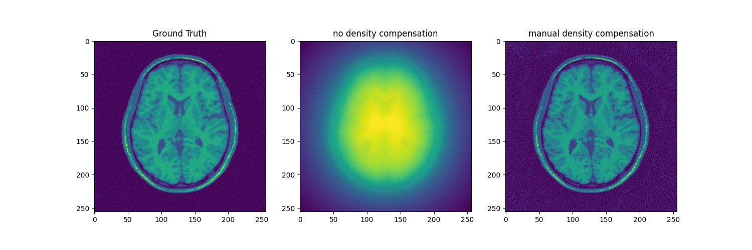
Manual Density Estimation

For some analytical trajectory it is also possible to determine the density compensation vector directly. In radial trajectory for instance, a sample’s weight can be determined from its distance to the center.

flat_traj = traj.reshape(-1, 2)
weights = np.sqrt(np.sum(flat_traj**2, axis=1))
nufft = get_operator("finufft")(traj, shape=mri_2D.shape, density=weights)
adjoint_manual = nufft.adj_op(kspace)
fig, axs = plt.subplots(1, 3, figsize=(15, 5))
axs[0].imshow(abs(mri_2D))
axs[0].set_title("Ground Truth")
axs[1].imshow(abs(adjoint))
axs[1].set_title("no density compensation")
axs[2].imshow(abs(adjoint_manual))
axs[2].set_title("manual density compensation")

/opt/hostedtoolcache/Python/3.10.14/x64/lib/python3.10/site-packages/mrinufft/_utils.py:87: UserWarning: Samples will be rescaled to [-pi, pi), assuming they were in [-0.5, 0.5)
  warnings.warn(

Text(0.5, 1.0, 'manual density compensation')

Operator-based method

Pipe’s Method

Pipe’s method is an iterative scheme, that use the interpolation and spreading kernel operator for computing the density compensation.

Warning

If this method is widely used in the literature, there exists no convergence guarantees for it.

Note

The Pipe method is currently only implemented for gpuNUFFT.

if check_backend("gpunufft"):
    flat_traj = traj.reshape(-1, 2)
    nufft = get_operator("gpunufft")(
        traj, shape=mri_2D.shape, density={"name": "pipe", "osf": 2}
    )
    adjoint_manual = nufft.adj_op(kspace)
    fig, axs = plt.subplots(1, 3, figsize=(15, 5))
    axs[0].imshow(abs(mri_2D))
    axs[0].set_title("Ground Truth")
    axs[1].imshow(abs(adjoint))
    axs[1].set_title("no density compensation")
    axs[2].imshow(abs(adjoint_manual))
    axs[2].set_title("Pipe density compensation")

    print(nufft.density)