
Note
Go to the end to download the full example code. or to run this example in your browser via Binder
Trajectory tools#
A collection of tools to manipulate and develop non-Cartesian trajectories.
Hereafter we detail and illustrate different generic tools that can be used and combined to create custom trajectories. Most of them are already present in the proposed trajectories from the literature. Since most arguments are redundant across the different patterns, some of the documentation will refer to previous patterns for explanation. Also note that not all possibilities are relevant for MR applications since these functions are only tools to simplify trajectory design.
In this page, we invite the user to manually run the script to be able to manipulate the plot orientations with the matplotlib interface to better visualize the 3D volumes.
# External
import matplotlib.pyplot as plt
import numpy as np
from utils import show_trajectories, show_trajectory

# Internal
import mrinufft as mn
import mrinufft.trajectories.tools as tools
from mrinufft.trajectories.utils import KMAX
Script options#
These options are used in the examples below as default values for all trajectories.
# Trajectory parameters
Nc = 80  # Number of shots
Ns = 500  # Number of samples per shot
in_out = True  # Choose between in-out or center-out trajectories
nb_repetitions = 8  # Number of stacks, rotations, cones, shells etc.
nb_revolutions = 1  # Number of revolutions for base trajectories
nb_zigzags = 5  # Number of zigzags for base trajectories

# Display parameters
figure_size = 10  # Figure size for trajectory plots
subfigure_size = 6  # Figure size for subplots
one_shot = 2 * Nc // 3  # Highlight one shot in particular
Direct tools#
In this section are presented the tools to apply over already instanciated trajectories, i.e. arrays of size \((N_c, N_s, N_d)\) with \(N_c\) the number of shots, \(N_s\) the number of samples per shot and \(N_d\) the number of dimensions (2 or 3).
Preparation#
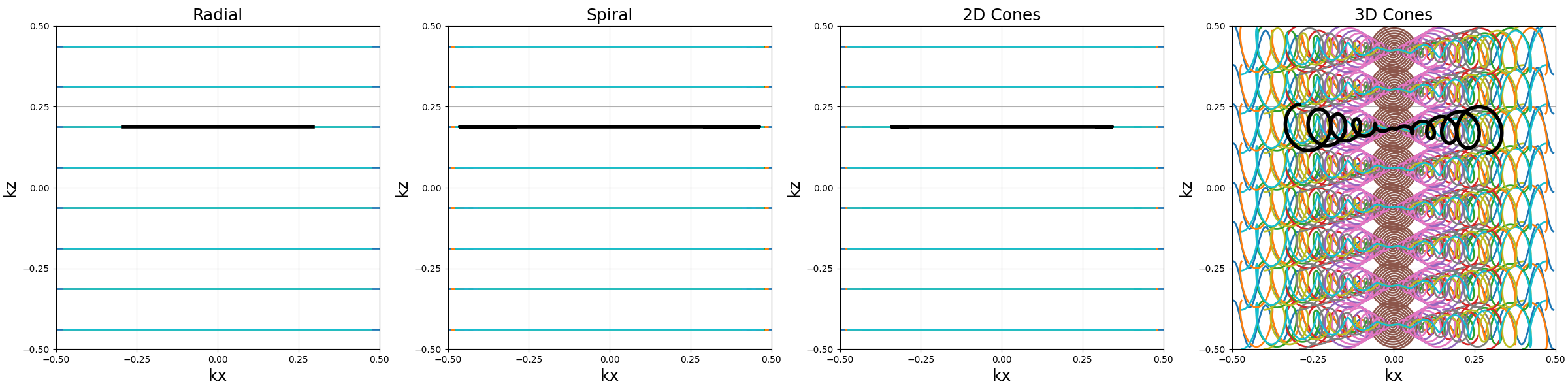
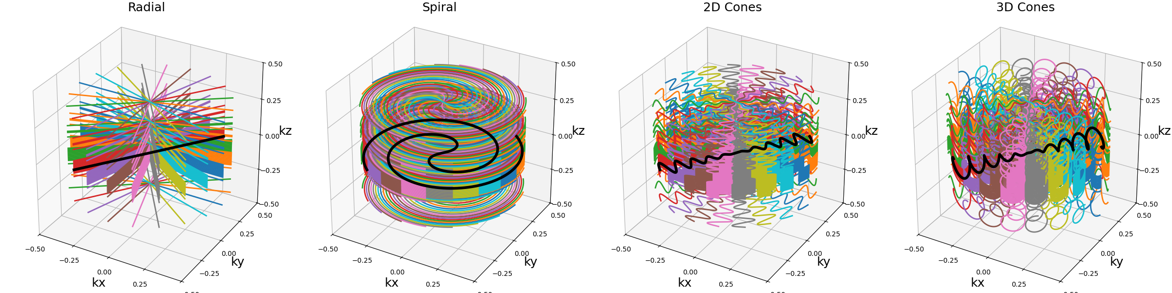
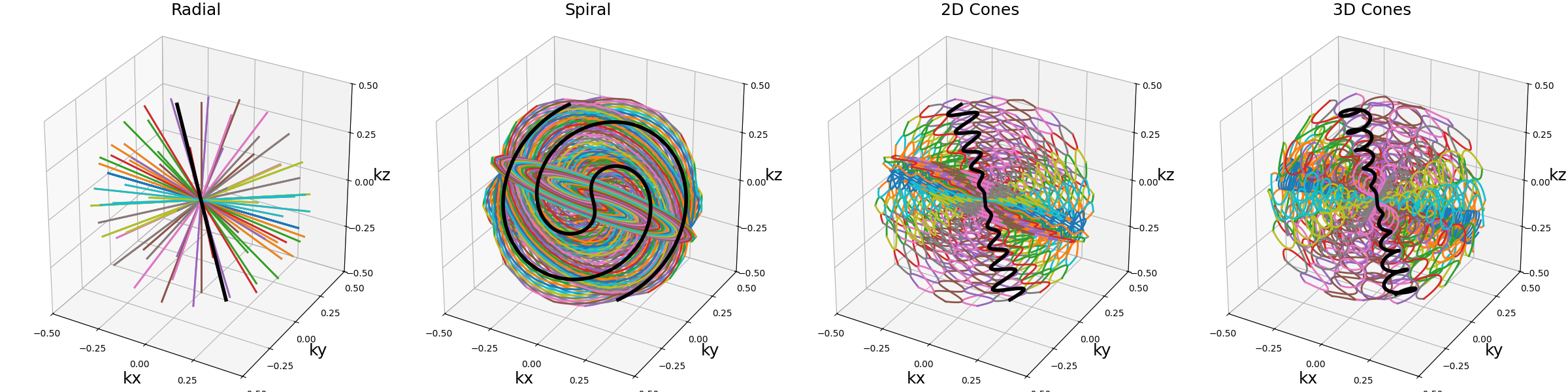
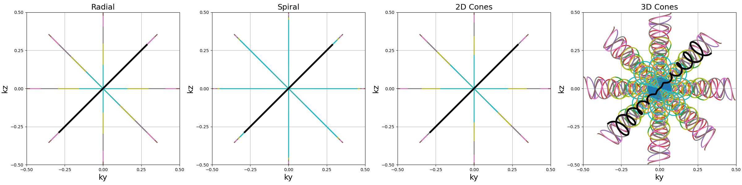
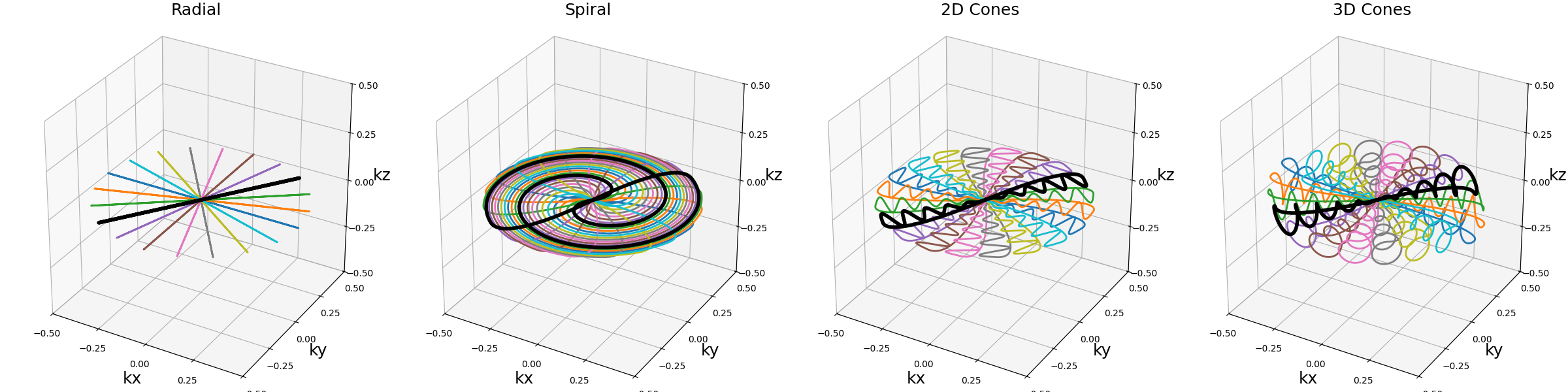
Single shots#
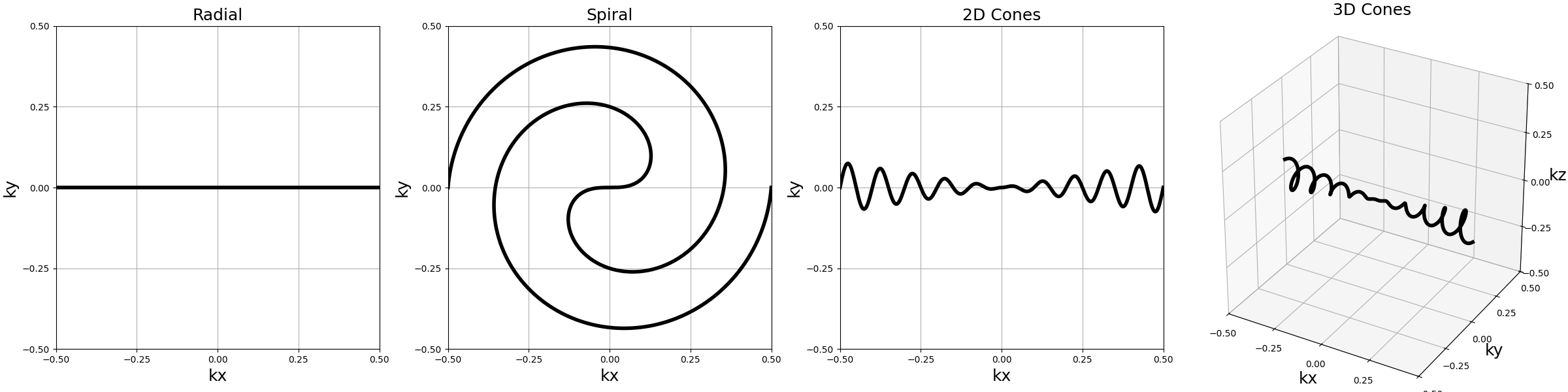
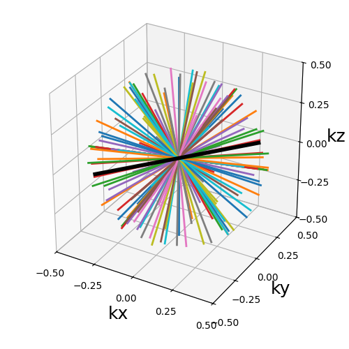
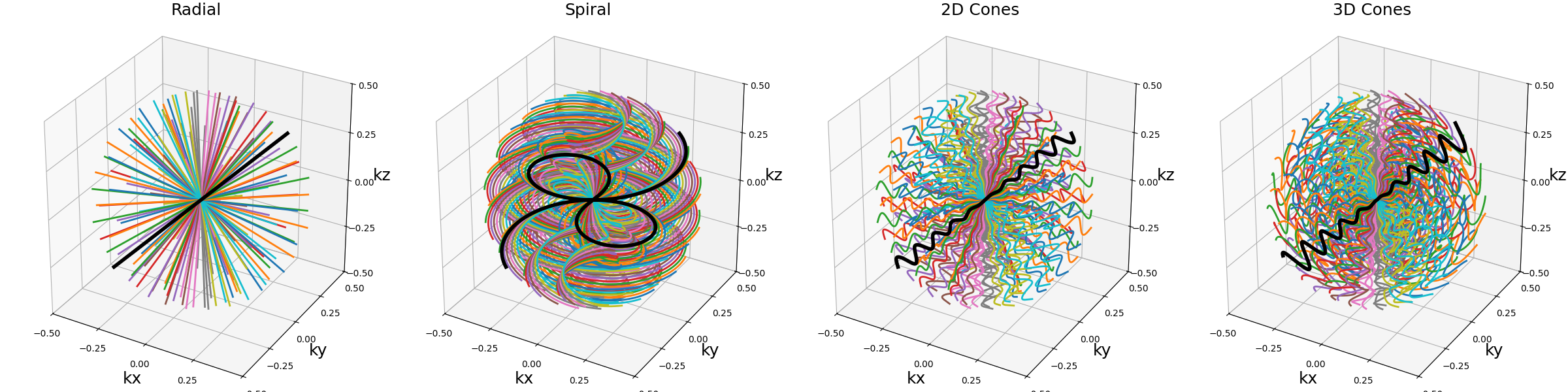
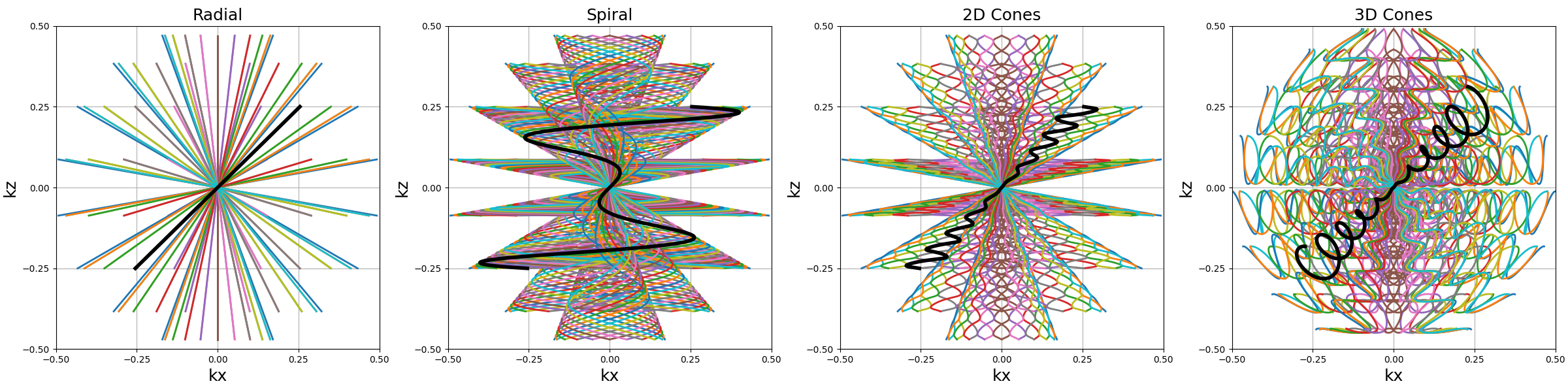
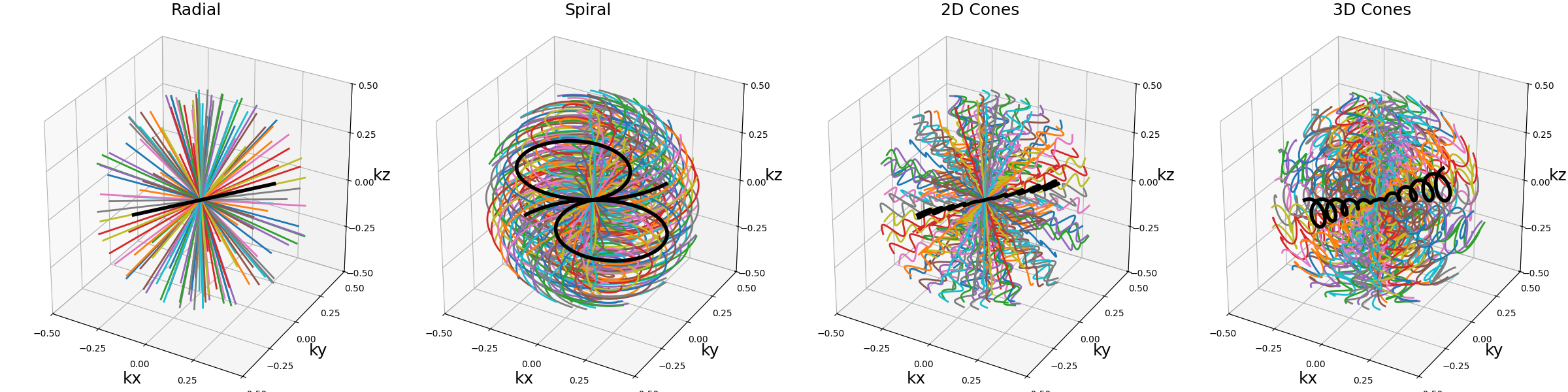
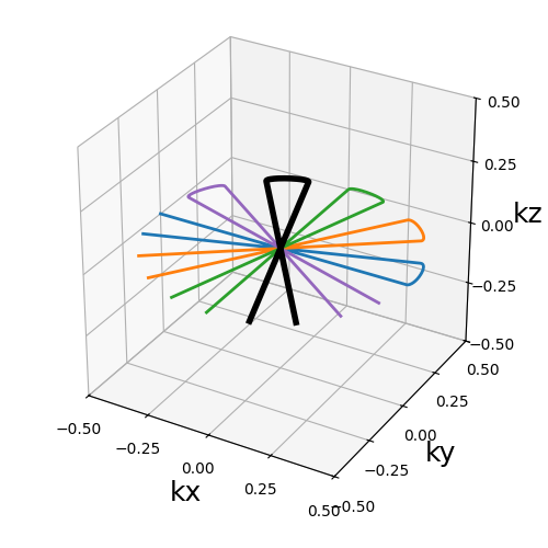
We can define a few simple trajectories to use in later examples: Single shots from 2D radial, Fermat’s spiral, and 2D/3D cones.
single_trajectories = {
    "Radial": mn.initialize_2D_radial(1, Ns, in_out=in_out),
    "Spiral": mn.initialize_2D_spiral(
        1, Ns, in_out=in_out, spiral="fermat", nb_revolutions=nb_revolutions
    ),
    "2D Cones": mn.initialize_2D_cones(
        Nc // nb_repetitions, Ns, in_out=in_out, nb_zigzags=nb_zigzags
    )[:1],
    "3D Cones": mn.initialize_3D_cones(Nc, Ns, in_out=in_out, nb_zigzags=nb_zigzags)[
        :1
    ],
}
arguments = ["Radial", "Spiral", "2D Cones", "3D Cones"]
function = lambda x: single_trajectories[x]
show_trajectories(
    function, arguments, one_shot=bool(one_shot), subfig_size=subfigure_size
)
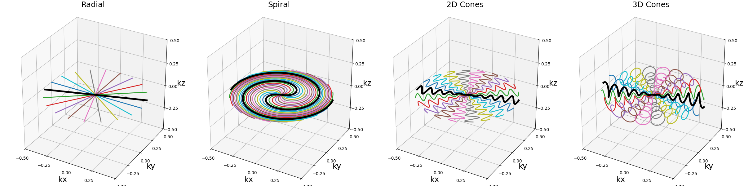
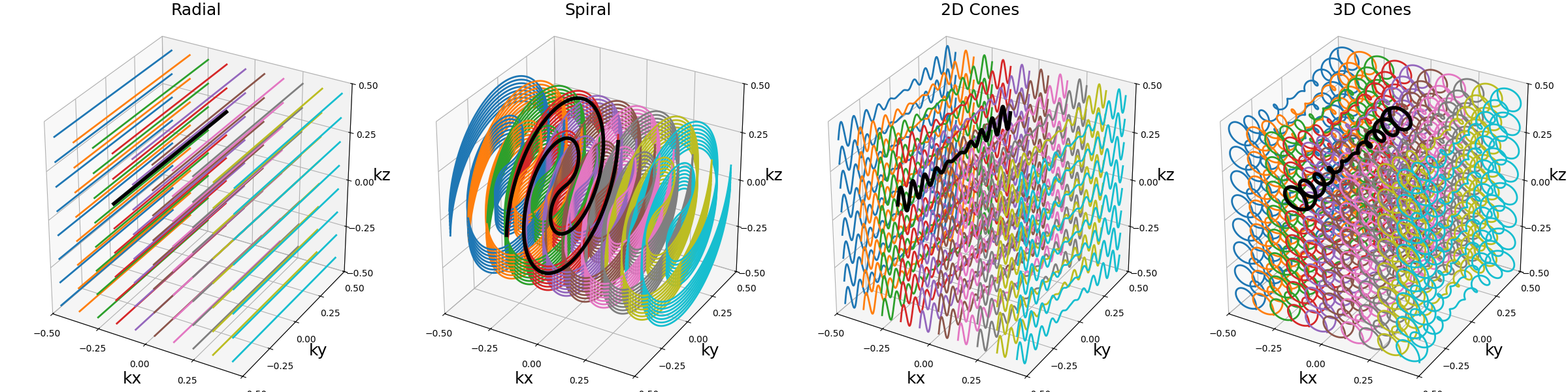
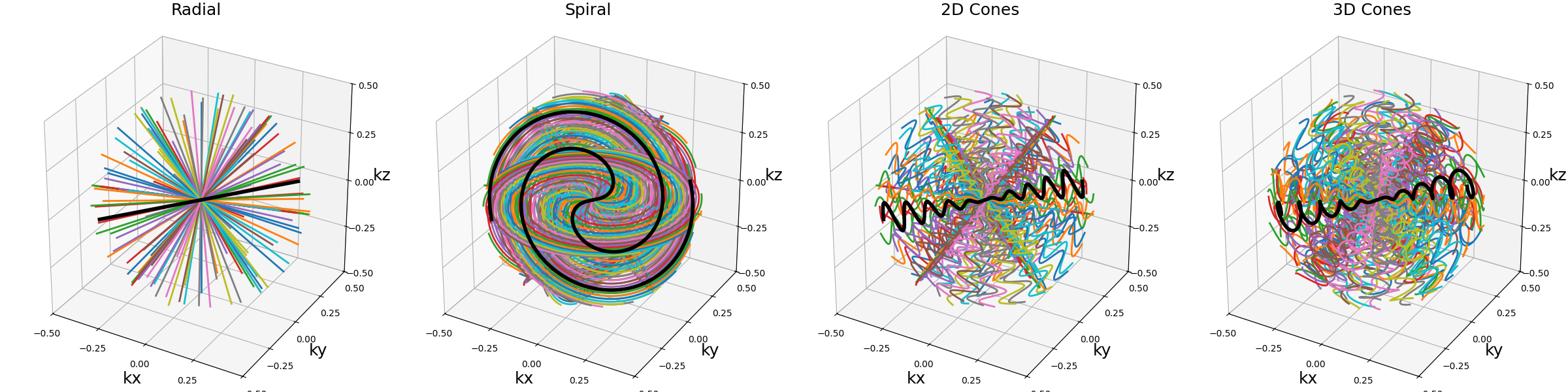
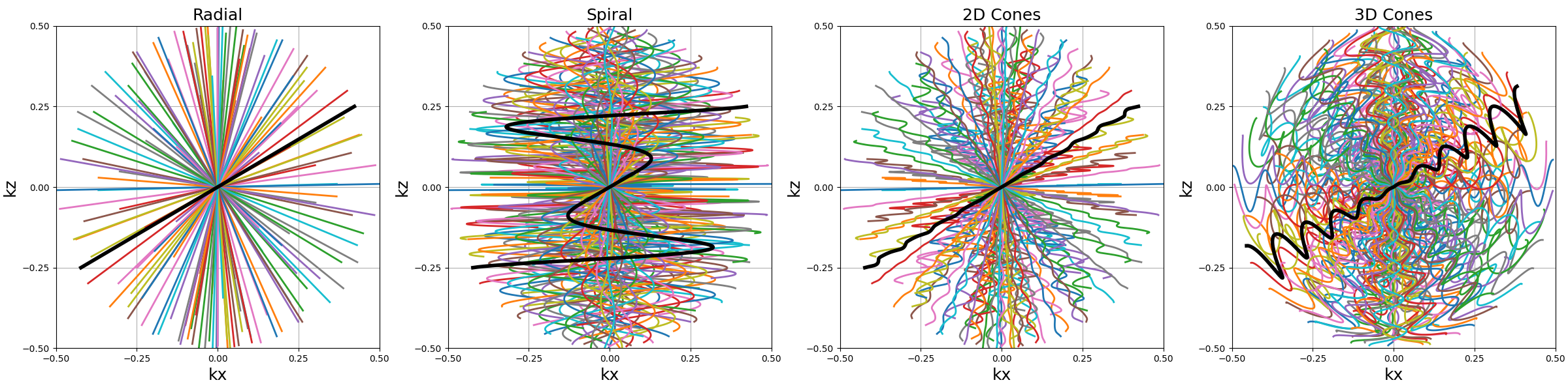
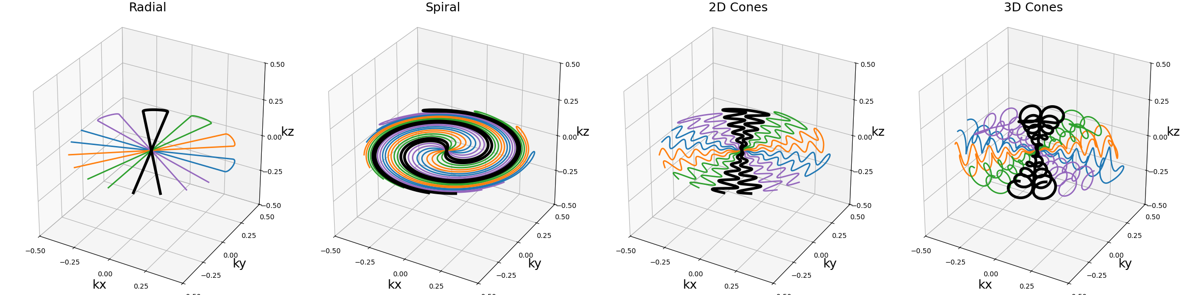
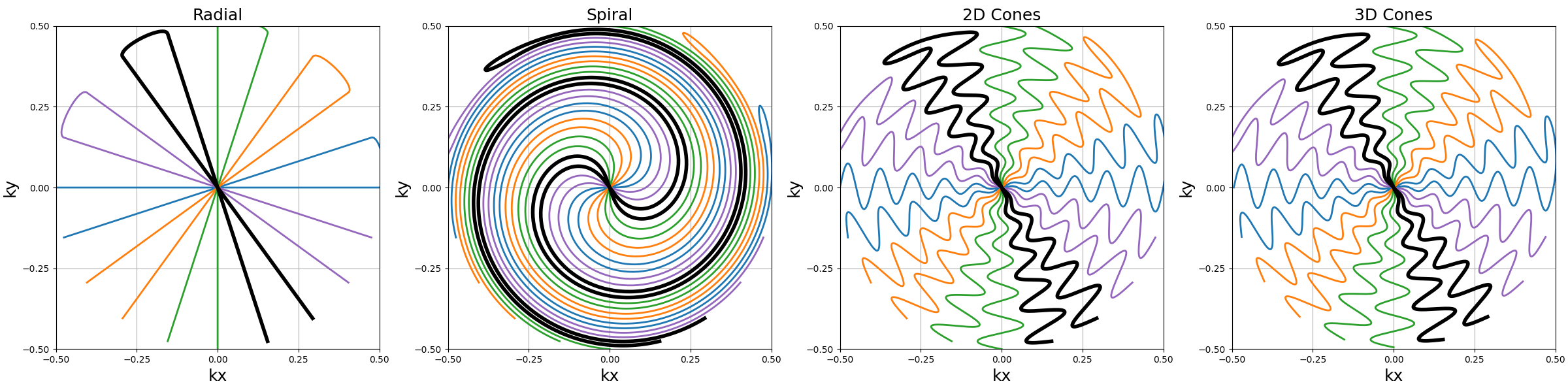
Planes#
We will also be using them as planes, or thick planes for 3D shots.
Nc_planes = Nc // nb_repetitions
z_tilt = 2 * np.pi / Nc_planes / (1 + in_out)

planar_trajectories = {
    "Radial": tools.rotate(
        single_trajectories["Radial"], nb_rotations=Nc_planes, z_tilt=z_tilt
    ),
    "Spiral": tools.rotate(
        single_trajectories["Spiral"], nb_rotations=Nc_planes, z_tilt=z_tilt
    ),
    "2D Cones": tools.rotate(
        single_trajectories["2D Cones"], nb_rotations=Nc_planes, z_tilt=z_tilt
    ),
    "3D Cones": tools.rotate(
        single_trajectories["3D Cones"], nb_rotations=Nc_planes, z_tilt=z_tilt
    ),
}
arguments = ["Radial", "Spiral", "2D Cones", "3D Cones"]
function = lambda x: planar_trajectories[x]
show_trajectories(
    function, arguments, one_shot=bool(one_shot), subfig_size=subfigure_size
)
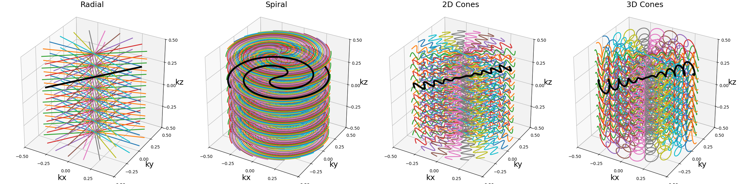
Stack#
The oldest and most widely used method is to simply stack any plane on top of itself, until it reaches the desired number of slices.
Arguments:
trajectory (array): array of k-space coordinates of size \((N_c, N_s, N_d)\)nb_stacks (int): number of stacks repeatingtrajectoryover the \(k_z\)-axis.z_tilt (float): angle tilt between consecutive stacks over the \(k_z\)-axis.(default None)hard_bounded (bool): whether the stacks should be strictly bounded to k-space.(default True)
trajectory = tools.stack(planar_trajectories["Radial"], nb_stacks=nb_repetitions)
show_trajectory(trajectory, figure_size=figure_size, one_shot=one_shot)
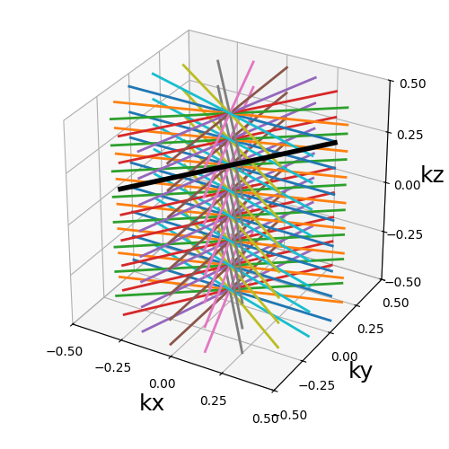
trajectory (array)#
The main use case is to stack trajectories consisting of flat or thick planes that will match the image slices. Some stacks can also be removed afterward to create GRAPPA-like patterns that will rely on parallel imaging and sensitivity maps to recover the missing information. Stacking planes without tilting them is notably compatible with stacked-NUFFT operators, reducing time and memory consumption during reconstruction.
arguments = ["Radial", "Spiral", "2D Cones", "3D Cones"]
function = lambda x: tools.stack(planar_trajectories[x], nb_stacks=nb_repetitions)
show_trajectories(function, arguments, one_shot=one_shot, subfig_size=subfigure_size)
show_trajectories(
    function,
    arguments,
    one_shot=one_shot,
    subfig_size=subfigure_size,
    dim="2D",
    axes=(0, 2),
)
It can also be applied twice to single shots to create a plane before stacking it over the \(k_z\)-axis. Note here that is does not make a lot of sense for non-radial trajectories such as spirals.
arguments = ["Radial", "Spiral", "2D Cones", "3D Cones"]
function = lambda x: tools.stack(
    np.roll(
        tools.stack(single_trajectories[x], nb_stacks=Nc_planes),
        axis=-1,
        shift=1,
    ),
    nb_stacks=nb_repetitions,
)
show_trajectories(function, arguments, one_shot=one_shot, subfig_size=subfigure_size)
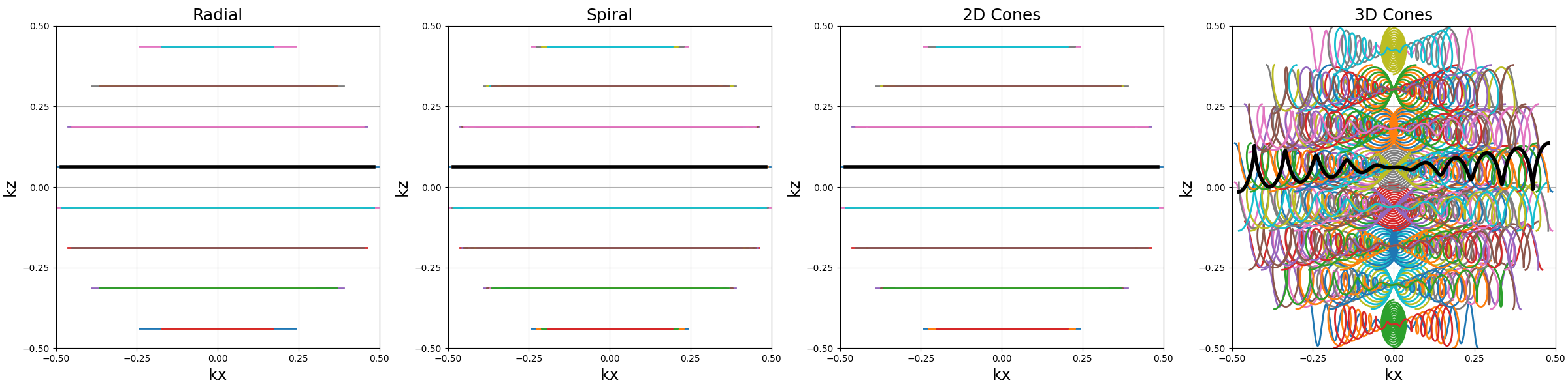
hard_bounded (bool)#
The stack is hard_bounded when the positions of the stacks
over the \(k_z\)-axis are squeezed such that the lower and upper
stacks don’t exceed the k-space boundaries when the plane is thick.
In the example below, the thickness is deliberately increased to
emphasize this point.
arguments = [True, False]
trajectory = np.copy(planar_trajectories["3D Cones"])
trajectory[..., 2] *= 2
function = lambda x: tools.stack(trajectory, nb_stacks=nb_repetitions, hard_bounded=x)
show_trajectories(
    function,
    arguments,
    one_shot=one_shot,
    subfig_size=subfigure_size,
    dim="2D",
    axes=(0, 2),
)
Stack Random#
A direct extension of the stacking expansion is to distribute the stacks according to a random distribution over the \(k_z\)-axis.
Arguments:
- trajectory (array): array of k-space coordinates of size
\((N_c, N_s, N_d)\)
- dim_size (int): size of the kspace in voxel units
- center_prop (int or float) : number of line
- acceleration (int): Acceleration factor
- pdf (str or array): Probability density function for the random distribution
- rng (int or np.random.Generator): Random number generator
- order (int): Order of the shots in the stack
trajectory = tools.stack_random(
    planar_trajectories["Spiral"],
    dim_size=128,
    center_prop=0.1,
    accel=16,
    pdf="uniform",
    order="top-down",
    rng=42,
)

show_trajectory(trajectory, figure_size=figure_size, one_shot=one_shot)
trajectory (array)#
The main use case is to stack trajectories consisting of flat or thick planes that will match the image slices.
arguments = ["Radial", "Spiral", "2D Cones", "3D Cones"]
function = lambda x: tools.stack_random(
    planar_trajectories[x],
    dim_size=128,
    center_prop=0.1,
    accel=16,
    pdf="gaussian",
    order="top-down",
    rng=42,
)
show_trajectories(function, arguments, one_shot=one_shot, subfig_size=subfigure_size)
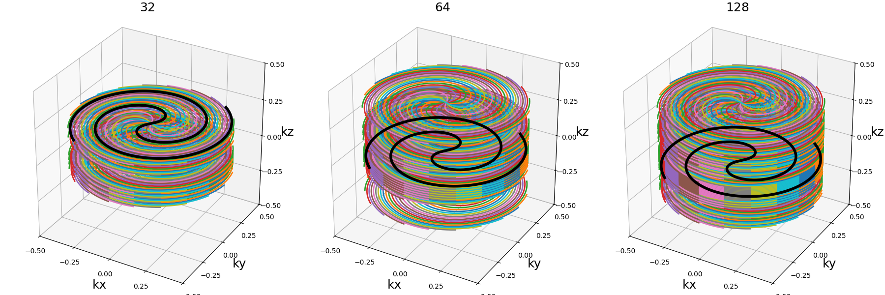
dim_size (int)#
Size of the k-space in voxel units over the stacking direction. It
is used to normalize the stack positions, and is used with the accel
factor and center_prop to determine the number of stacks.
arguments = [32, 64, 128]
function = lambda x: tools.stack_random(
    planar_trajectories["Spiral"],
    dim_size=x,
    center_prop=0.1,
    accel=8,
    pdf="gaussian",
    order="top-down",
    rng=42,
)
show_trajectories(function, arguments, one_shot=one_shot, subfig_size=subfigure_size)
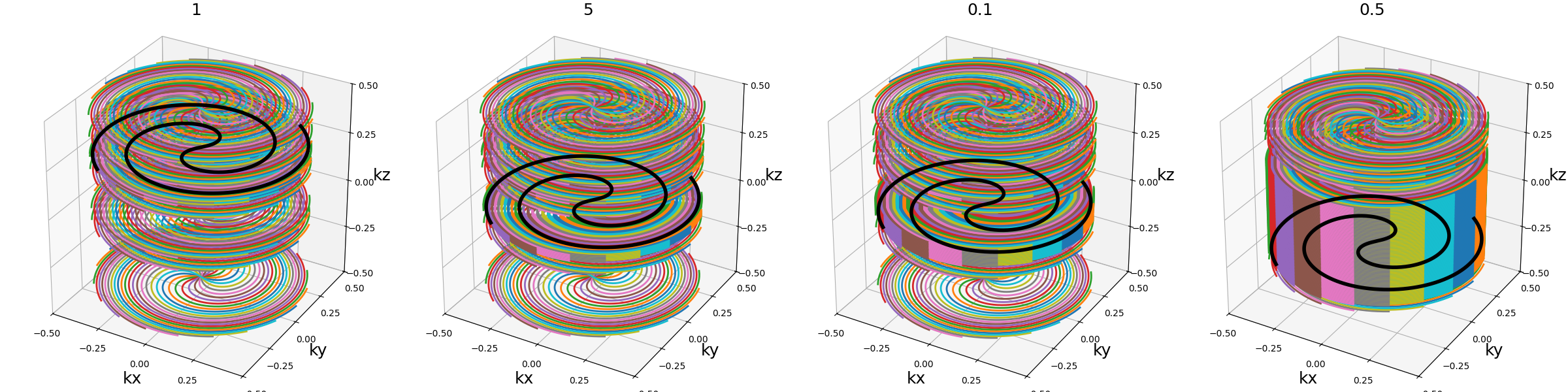
center_prop (int or float)#
Number of lines to keep in the center of the k-space. It is used to determine
the number of stacks and the acceleration factor, and to keep the center of
the k-space with a higher density of shots. If a float this is a fraction
of the total dim_size. If int it is directly the number of lines.
arguments = [1, 5, 0.1, 0.5]
function = lambda x: tools.stack_random(
    planar_trajectories["Spiral"],
    dim_size=128,
    center_prop=x,
    accel=16,
    pdf="uniform",
    order="top-down",
    rng=42,
)
show_trajectories(function, arguments, one_shot=one_shot, subfig_size=subfigure_size)
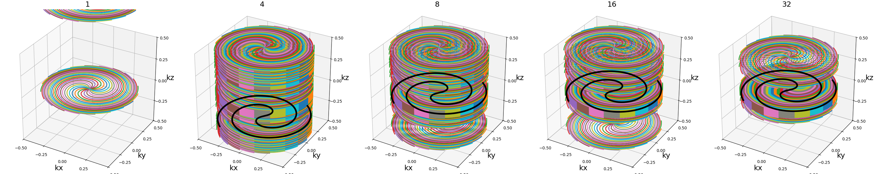
accel (int)#
Acceleration factor to subsample the outer region of the k-space. Note that the acceleration factor does not take into account the center lines.
arguments = [1, 4, 8, 16, 32]
function = lambda x: tools.stack_random(
    planar_trajectories["Spiral"],
    dim_size=128,
    center_prop=0.1,
    accel=x,
    pdf="uniform",
    order="top-down",
    rng=42,
)
show_trajectories(function, arguments, one_shot=one_shot, subfig_size=subfigure_size)
pdf (str or array)#
Probability density function for the sampling of the outer region. It can
either be a string to use a known probability law (“gaussian” or “uniform”) or
“equispaced” for a coherent undersampling (like the one used in GRAPPA). It
can also be a array, for using a customed density probability.
In this case, it will be normalized so that sum(pdf) =1.
dim_size = 128
arguments = [
    "gaussian",
    "uniform",
    "equispaced",
    np.arange(dim_size),
]
function = lambda x: tools.stack_random(
    planar_trajectories["Spiral"],
    dim_size=128,
    center_prop=0.1,
    accel=32,
    pdf=x,
    order="top-down",
    rng=42,
)
show_trajectories(function, arguments, one_shot=one_shot, subfig_size=subfigure_size)
![gaussian, uniform, equispaced, [ 0 1 2 3 4 5 6 7 8 9 10 11 12 13 14 15 16 17 18 19 20 21 22 23 24 25 26 27 28 29 30 31 32 33 34 35 36 37 38 39 40 41 42 43 44 45 46 47 48 49 50 51 52 53 54 55 56 57 58 59 60 61 62 63 64 65 66 67 68 69 70 71 72 73 74 75 76 77 78 79 80 81 82 83 84 85 86 87 88 89 90 91 92 93 94 95 96 97 98 99 100 101 102 103 104 105 106 107 108 109 110 111 112 113 114 115 116 117 118 119 120 121 122 123 124 125 126 127]](../../_images/sphx_glr_example_trajectory_tools_013.png)
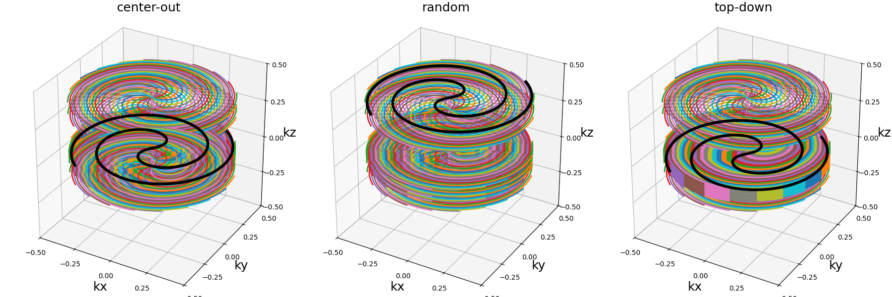
order (str)#
Determine the ordering of the shot in the trajectory. Accepeted values are “center-out”, “top-down” or “random”.
dim_size = 128
arguments = [
    "center-out",
    "random",
    "top-down",
]
function = lambda x: tools.stack_random(
    planar_trajectories["Spiral"],
    dim_size=128,
    center_prop=0.1,
    accel=32,
    pdf="uniform",
    order=x,
    rng=42,
)
show_trajectories(function, arguments, one_shot=one_shot, subfig_size=subfigure_size)
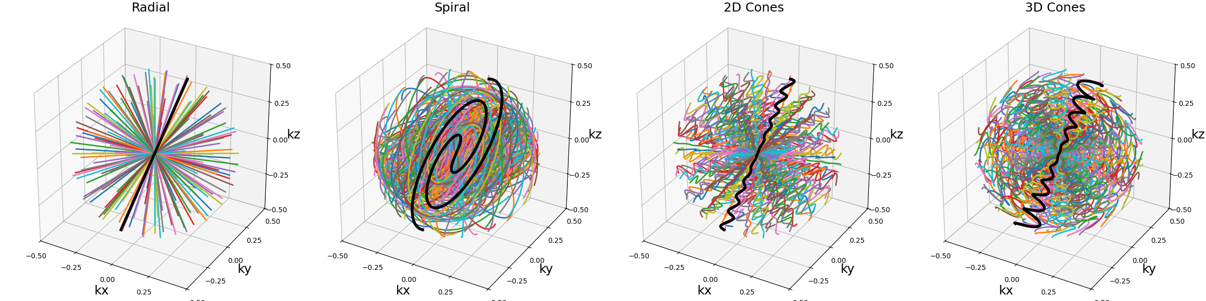
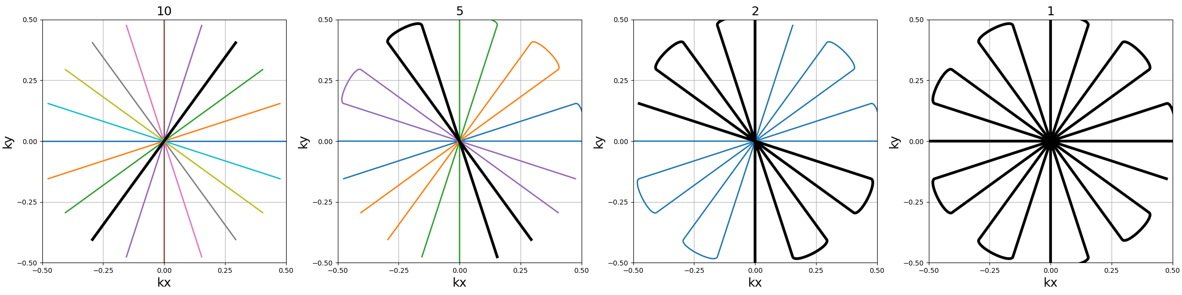
Rotate#
A simple method to duplicate any trajectory with a rotation over one or multiple axes at the same time.
Arguments:
trajectory (array): array of k-space coordinates of size \((N_c, N_s, N_d)\)nb_rotations (int): number of rotations repeatingtrajectory.x_tilt (float): angle tilt between consecutive stacks over the \(k_x\)-axis.(default None)y_tilt (float): angle tilt between consecutive stacks over the \(k_y\)-axis.(default None)z_tilt (float): angle tilt between consecutive stacks over the \(k_z\)-axis.(default None)
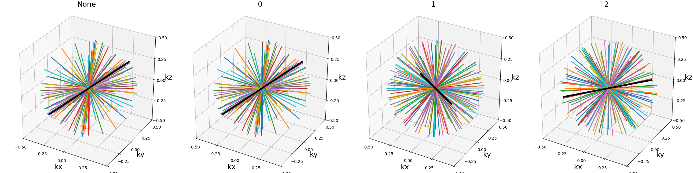
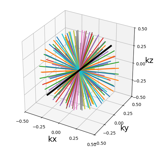
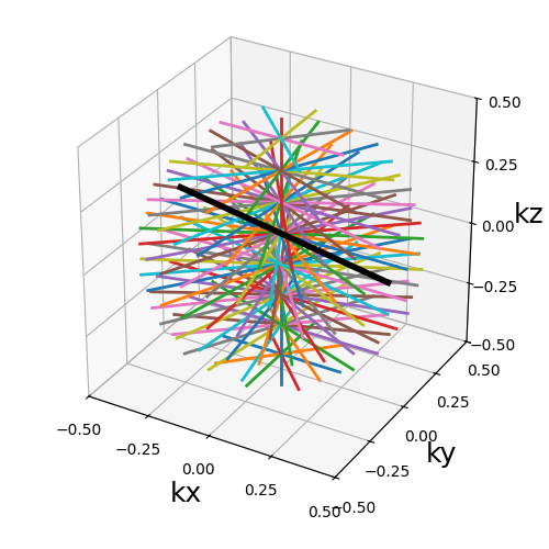
trajectory = tools.rotate(
    planar_trajectories["Radial"], nb_rotations=nb_repetitions, x_tilt="uniform"
)
show_trajectory(trajectory, figure_size=figure_size, one_shot=one_shot)
trajectory (array)#
A common application is to rotate a single shot to create a plane as used earlier to initialize the planar trajectories. It has also been used in the literature to rotate planes around one axis to create 3D trajectories, but the density (and redundancy) along that axis is then much greater than anywhere else.
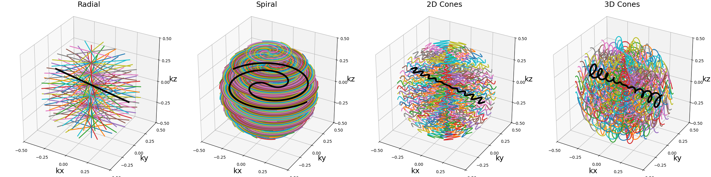
arguments = ["Radial", "Spiral", "2D Cones", "3D Cones"]
function = lambda x: tools.rotate(
    planar_trajectories[x],
    nb_rotations=nb_repetitions,
    x_tilt="uniform",
)
show_trajectories(function, arguments, one_shot=one_shot, subfig_size=subfigure_size)
show_trajectories(
    function,
    arguments,
    one_shot=one_shot,
    subfig_size=subfigure_size,
    dim="2D",
    axes=(1, 2),
)
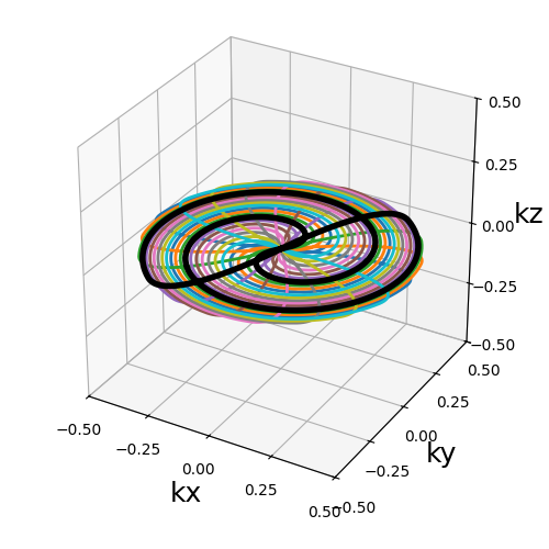
Precess#
A method to duplicate a trajectory while applying a precession-like rotation around a provided axis.
Arguments:
trajectory (array): array of k-space coordinates of size \((N_c, N_s, N_d)\)nb_rotations (int): number of rotations repeatingtrajectoryover the \(k_z\)-axis.tilt (float): angle tilt between consecutive rotations around the \(k_z\)-axis.(default "golden")half_sphere (bool): whether the precession should be limited to the upper half of the k-space sphere, typically for in-out trajectories or planes.(default False)partition (str): partition type between an “axial” or “polar” split of the \(k_z\)-axis, designating whether the axis should be fragmented by radius or angle respectively.(default "axial")axis (int, array): axis selected for alignment reference when rotating the trajectory around the \(k_z\)-axis, generally corresponding to the shot direction for single shottrajectoryinputs. It can either be an integer for one of the three k-space axes, or directly a 3D array. The default behavior whenNoneis to select the last coordinate of the first shot as the axis.(default None)
trajectory = tools.precess(
    planar_trajectories["Radial"],
    nb_rotations=nb_repetitions,
    tilt="golden",
    half_sphere=in_out,
    axis=2,
)
show_trajectory(trajectory, figure_size=figure_size, one_shot=one_shot)
trajectory (array)#
This method provides a way to distribute duplicated trajectories (single shots, planes or anything else) to cover evenly a provided axis tilting the azimuthal orientation.
arguments = ["Radial", "Spiral", "2D Cones", "3D Cones"]
function = lambda x: tools.precess(
    planar_trajectories[x],
    nb_rotations=nb_repetitions,
    tilt="golden",
    half_sphere=in_out,
    axis=2,
)
show_trajectories(function, arguments, one_shot=one_shot, subfig_size=subfigure_size)
It is however most often used with single shots to cover more evenly the k-space sphere, such as with 3D cones or Seiffert spirals. Indeed, applying a precession with the golden angle is known to approximate an even distribution of points over a sphere surface.
arguments = ["Radial", "Spiral", "2D Cones", "3D Cones"]
function = lambda x: tools.precess(
    single_trajectories[x],
    nb_rotations=Nc,
    tilt="golden",
    half_sphere=in_out,
    axis=0,
)
show_trajectories(function, arguments, one_shot=one_shot, subfig_size=subfigure_size)
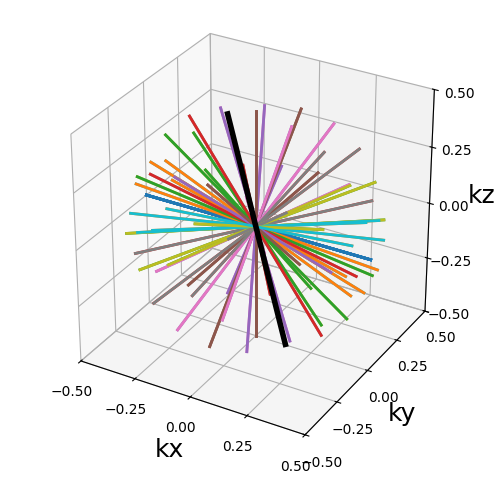
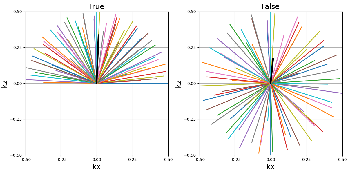
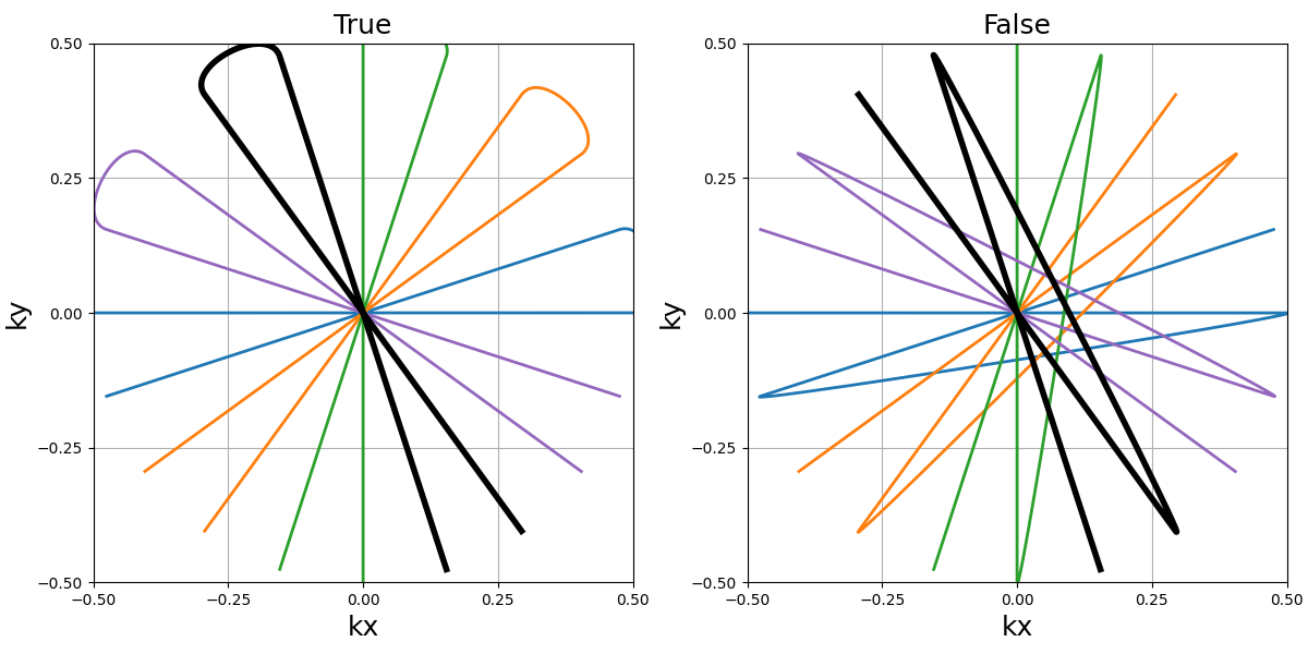
half_sphere (bool)#
Whether the precession should be limited to the upper half of the k-space sphere (with respect to the provided axis). It is typically used for in-out trajectories or planes, as otherwise shots would likely be stacked in a redundant way.
In the example hereafter, center-out shots are shown for clarity.
arguments = [True, False]
function = lambda x: tools.precess(
    single_trajectories["Radial"][:, Ns // (1 + in_out) :],
    nb_rotations=Nc,
    tilt="golden",
    half_sphere=x,
    axis=0,
)
show_trajectories(
    function,
    arguments,
    one_shot=one_shot,
    subfig_size=subfigure_size,
    dim="2D",
    axes=(0, 2),
)
partition (str)#
Partition type between an “axial” or “polar” split of the \(k_z\)-axis, designating whether the axis should be fragmented by radius or angle respectively.
arguments = ["axial", "polar"]
function = lambda x: tools.precess(
    single_trajectories["Radial"],
    nb_rotations=Nc,
    tilt=None,
    partition=x,
    axis=0,
)
show_trajectories(
    function,
    arguments,
    one_shot=one_shot,
    subfig_size=subfigure_size,
    dim="2D",
    axes=(0, 2),
)
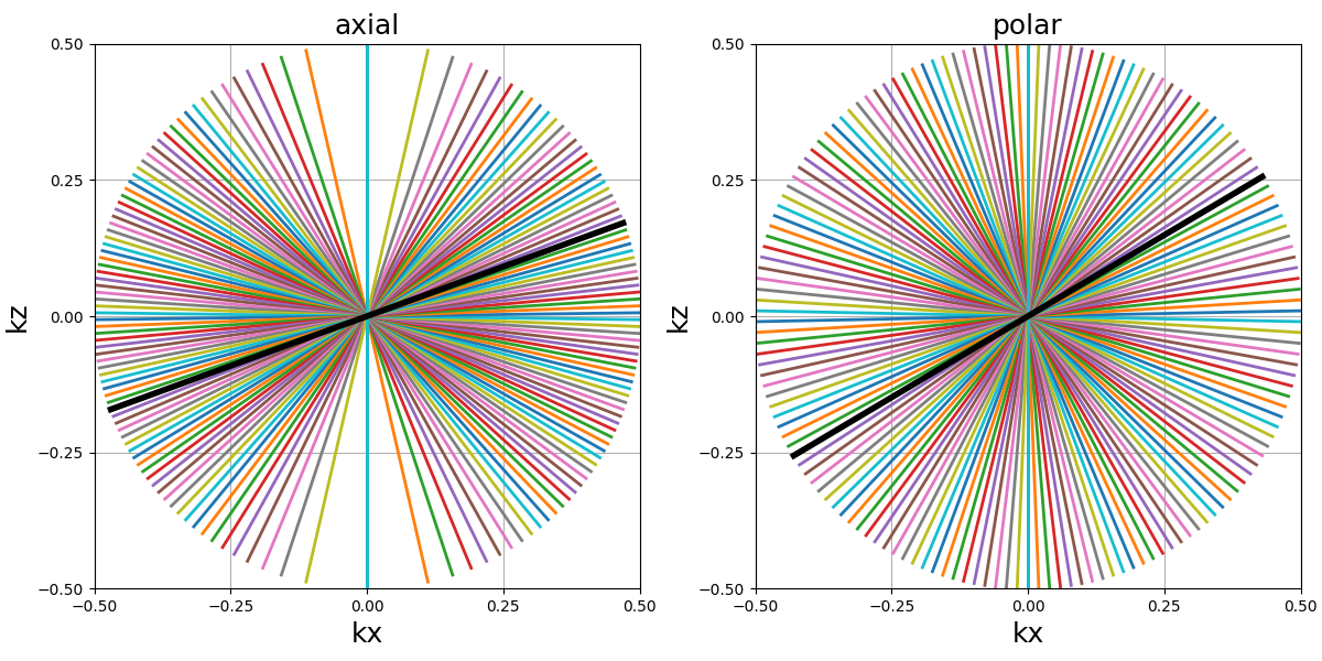
While “polar” looks more natural in the absence of rotation (tilt=None),
it results in too many shots close to the rotation axis, and therefore
a non-uniform density. The best approximation of a uniform distribution
is obtained with an “axial” partition and “golden” tilt along
the provided axis.
arguments = ["axial", "polar"]
function = lambda x: tools.precess(
    single_trajectories["Radial"],
    nb_rotations=Nc,
    tilt="golden",
    partition=x,
    axis=0,
)
show_trajectories(
    function,
    arguments,
    one_shot=one_shot,
    subfig_size=subfigure_size,
    dim="2D",
    axes=(0, 2),
)
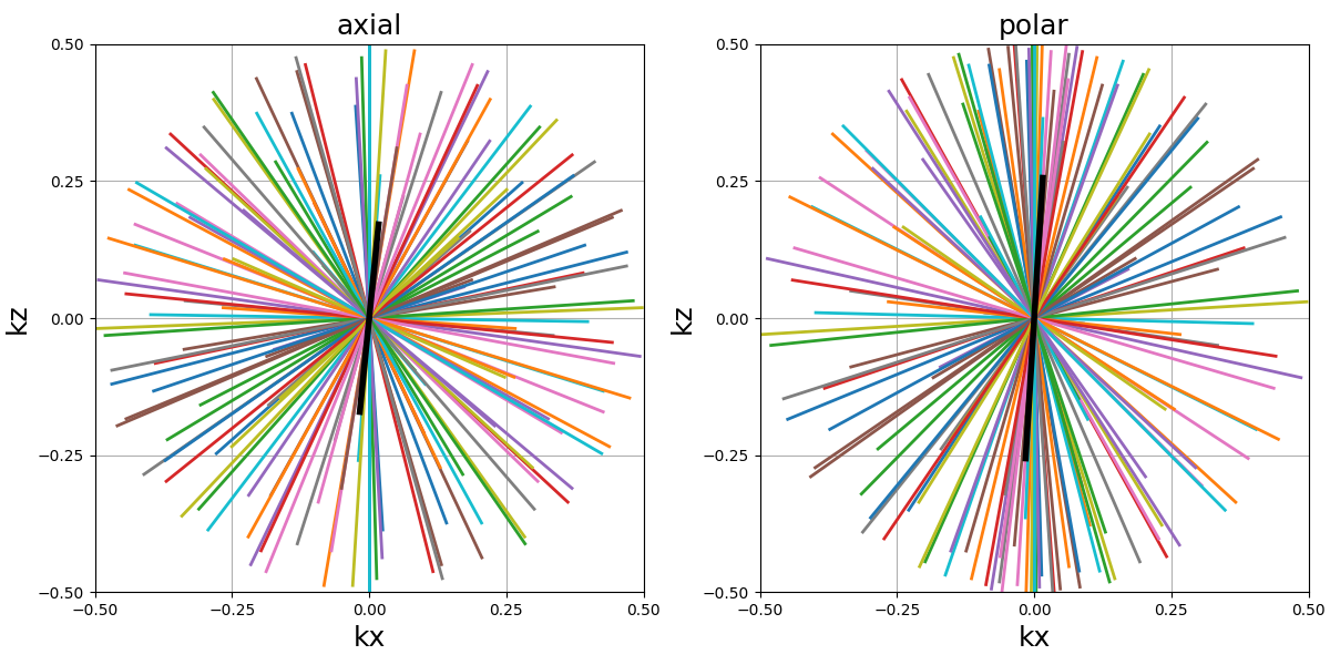
The distribution over the k-space sphere surface can be shown by displaying only the tip of the shots.
arguments = ["axial", "polar"]
function = lambda x: tools.precess(
    single_trajectories["Radial"][:, -5:],
    nb_rotations=Nc,
    tilt="golden",
    partition=x,
    axis=0,
)
show_trajectories(function, arguments, one_shot=one_shot, subfig_size=subfigure_size)
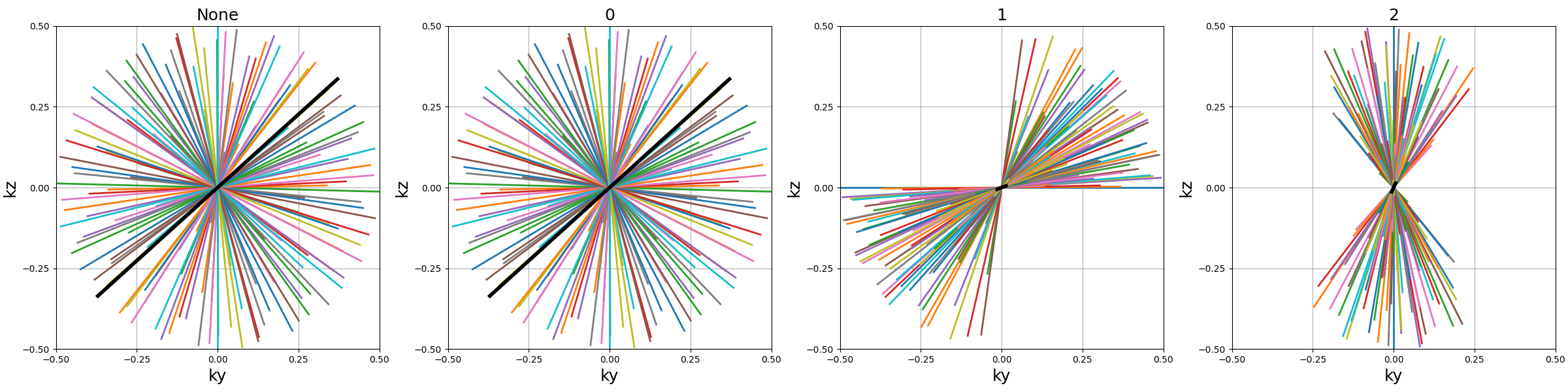
axis (int, array)#
Axis selected for alignment reference when rotating the trajectory
around the \(k_z\)-axis, generally corresponding to the
shot direction for single shot trajectory inputs.
It can either be an integer for one of the three k-space axes,
or directly a 3D array. The default behavior when None
is to select the last coordinate of the first shot as the axis.
This argument is simple to select but still important, as the precession relies on Rodrigues’ rotation coefficients that enable a rotation from one vector to another to align the trajectory through the provided axis with the precession vectors all over the k-space sphere. However, misalignement between shots and the provided axis will result in a non-uniform distribution, as the rotation around the axis is unfavorably deterministic.
The first case is single shots, where the provided axis should simply correspond to the shot axis.
arguments = [None, 0, 1, 2]
function = lambda x: tools.precess(
    single_trajectories["Radial"],
    nb_rotations=Nc,
    tilt="golden",
    half_sphere=in_out,
    axis=x,
)
show_trajectories(
    function,
    arguments,
    one_shot=one_shot,
    subfig_size=subfigure_size,
    dim="2D",
    axes=(1, 2),
)
The second case is planar trajectories, where the axis orthogonal to the shots plane is preferred.
arguments = [None, 0, 1, 2]
function = lambda x: tools.precess(
    planar_trajectories["Radial"],
    nb_rotations=nb_repetitions,
    tilt="golden",
    half_sphere=in_out,
    axis=x,
)
show_trajectories(function, arguments, one_shot=one_shot, subfig_size=subfigure_size)
Some trickier cases exist in the literature, with the example of Seiffert spirals. Those 3D spirals neither correspond to a single-axis shot or a plane, so the authors chose to use the center-out axis of each shot as a reference axis for the rotation. In order to handle the redundant distribution, they added a pseudo-random rotation within the shot axes.
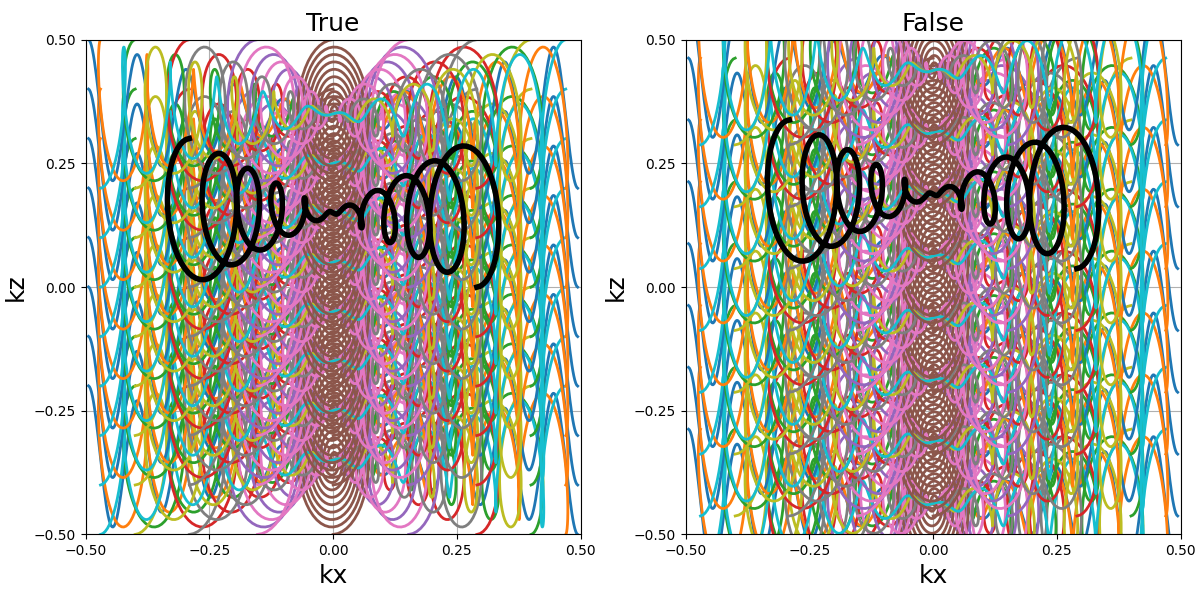
Conify#
A tool to distort trajectories into multiple cones positioned to cover the k-space sphere.
Arguments:
trajectory (array): array of k-space coordinates of size \((N_c, N_s, N_d)\)nb_cones (int): number of cones repeatingtrajectorywith conical distortion over the \(k_z\)-axis.z_tilt (float): angle tilt between consecutive cones around the \(k_z\)-axis.(default "golden")in_out (bool): whether to account for the in-out nature of some trajectories to avoid hard angles around the center,(default False)max_angle (float): maximum angle of the cones.(default pi / 2)borderless (bool): Whether the cones should reach max_angle or not, mostly to avoid 1D cones ifmax_angleis equal to pi / 2, by default True.
trajectory = tools.conify(
    planar_trajectories["Radial"], nb_cones=nb_repetitions, in_out=in_out
)
show_trajectory(trajectory, figure_size=figure_size, one_shot=one_shot)
trajectory (array)#
The trajectory is folded toward the \(k_z\)-axis to shape cones, and is therefore expected to be planar over the \(k_x-k_y\) axes. Other configuration might result in irrelevant trajectories. Also, the distortion is likely to increase the required gradient amplitudes and slew rates.
arguments = ["Radial", "Spiral", "2D Cones", "3D Cones"]
function = lambda x: tools.conify(
planar_trajectories[x], nb_cones=nb_repetitions, in_out=in_out
)
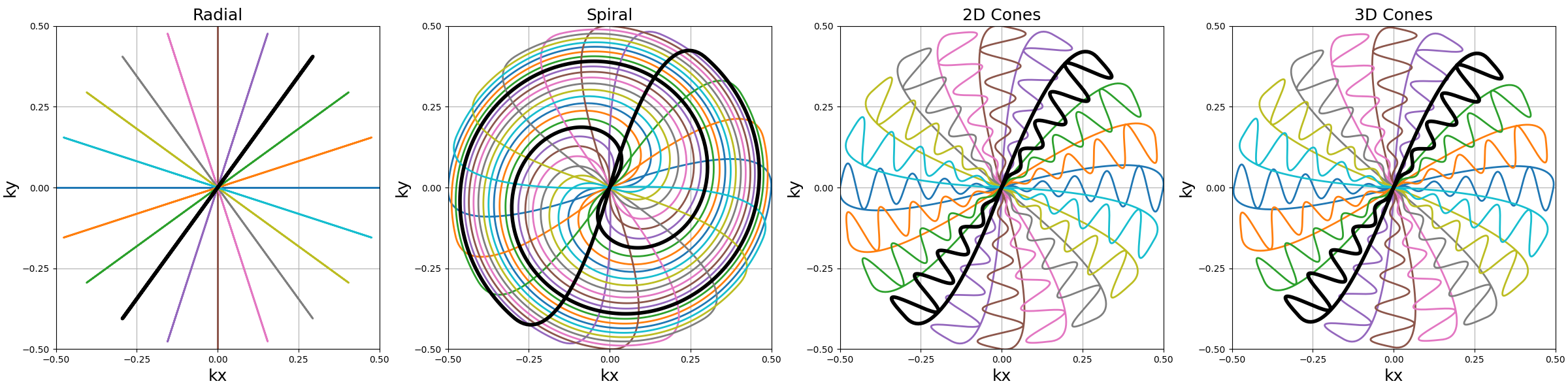
show_trajectories(function, arguments, one_shot=one_shot, subfig_size=subfigure_size)
show_trajectories(
    function,
    arguments,
    one_shot=one_shot,
    subfig_size=subfigure_size,
    dim="2D",
    axes=(0, 2),
)
Similarly to other tools, it can be used with single shots.
In that case, nb_cones is set to Nc to create as many
individual cones.
arguments = ["Radial", "Spiral", "2D Cones", "3D Cones"]
function = lambda x: tools.conify(
    single_trajectories[x], nb_cones=Nc, z_tilt="golden", in_out=in_out
)
show_trajectories(function, arguments, one_shot=one_shot, subfig_size=subfigure_size)
show_trajectories(
    function,
    arguments,
    one_shot=one_shot,
    subfig_size=subfigure_size,
    dim="2D",
    axes=(0, 2),
)
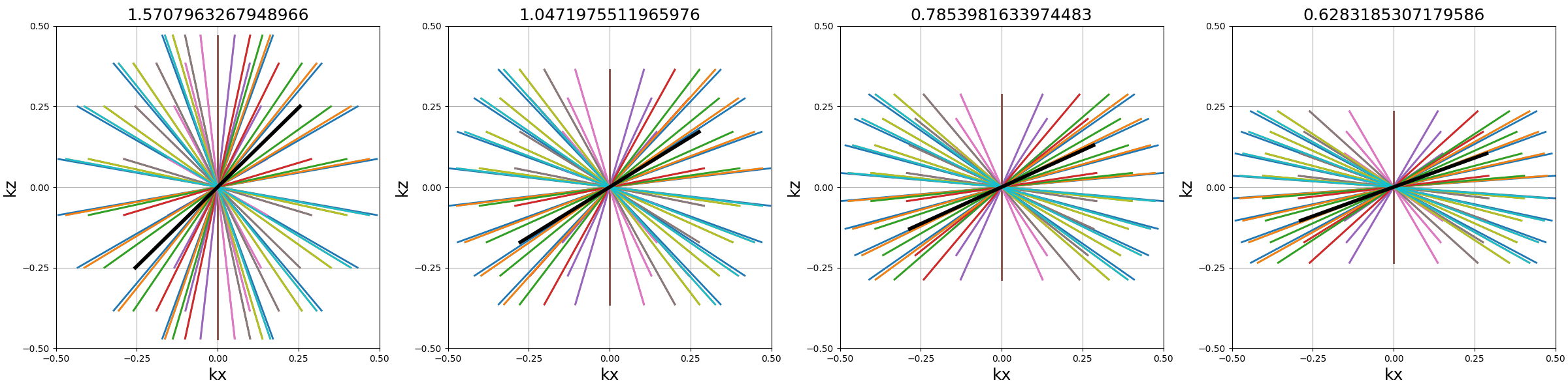
max_angle (float)#
Polar angle of the most folded cone. As pointed out in [Pip+11], folding planes over the whole sphere would result in inefficient distributions near the \(k_z\)-axis, and it may be more relevant to reduce the maximum angle but duplicate all of the cones along another axis to still cover the whole k-space.
arguments = [np.pi / 2, np.pi / 3, np.pi / 4, np.pi / 5]
function = lambda x: tools.conify(
    planar_trajectories["Radial"],
    nb_cones=nb_repetitions,
    in_out=in_out,
    max_angle=x,
)
show_trajectories(
    function,
    arguments,
    one_shot=one_shot,
    subfig_size=subfigure_size,
    dim="2D",
    axes=(0, 2),
)
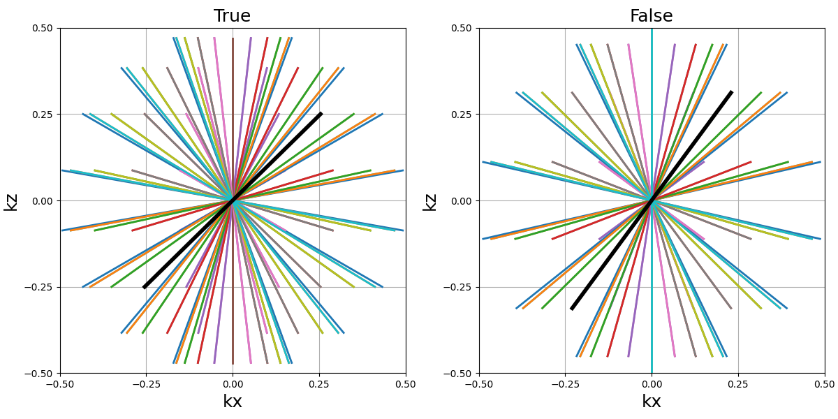
borderless (bool)#
Define whether or not the edge cones should reach max_angle
when equal to False, or instead simply partition the
sphere over a polar split.
arguments = [True, False]
function = lambda x: tools.conify(
    planar_trajectories["Radial"],
    nb_cones=nb_repetitions,
    in_out=in_out,
    max_angle=np.pi / 2,
    borderless=x,
)
show_trajectories(
    function,
    arguments,
    one_shot=one_shot,
    subfig_size=subfigure_size,
    dim="2D",
    axes=(0, 2),
)
Epify#
A tool to assemble multiple single-readout shots together by adding transition steps in the trajectory to create EPI-like multi-readout shots.
Note that the epify tool is associated with an unepify
tool to revert the operation on trajectory or acquired data.
Arguments:
trajectory (array_like): trajectory to change by prolonging and merging the shots together.Ns_transitions (int): number of samples/steps between the merged readouts.nb_trains (int): number of resulting multi-readout shots, or trains.reverse_odd_shots (bool): Whether to reverse every odd shots such that, as in most trajectories, even shots end up closer to the start of odd shots.
trajectory = tools.epify(
    planar_trajectories["Radial"],
    Ns_transitions=Ns // 10,
    nb_trains=Nc_planes // 2,
    reverse_odd_shots=True,
)
show_trajectory(trajectory, figure_size=figure_size, one_shot=one_shot)
trajectory (array)#
The trajectory to change by prolonging and merging the shots together. Hereafter the shots are merged by pairs with short transitions.
arguments = ["Radial", "Spiral", "2D Cones", "3D Cones"]
function = lambda x: tools.epify(
    planar_trajectories[x],
    Ns_transitions=Ns // 10,
    nb_trains=Nc_planes // 2,
    reverse_odd_shots=True,
)
show_trajectories(function, arguments, one_shot=one_shot, subfig_size=subfigure_size)
show_trajectories(
    function, arguments, one_shot=one_shot, subfig_size=subfigure_size, dim="2D"
)
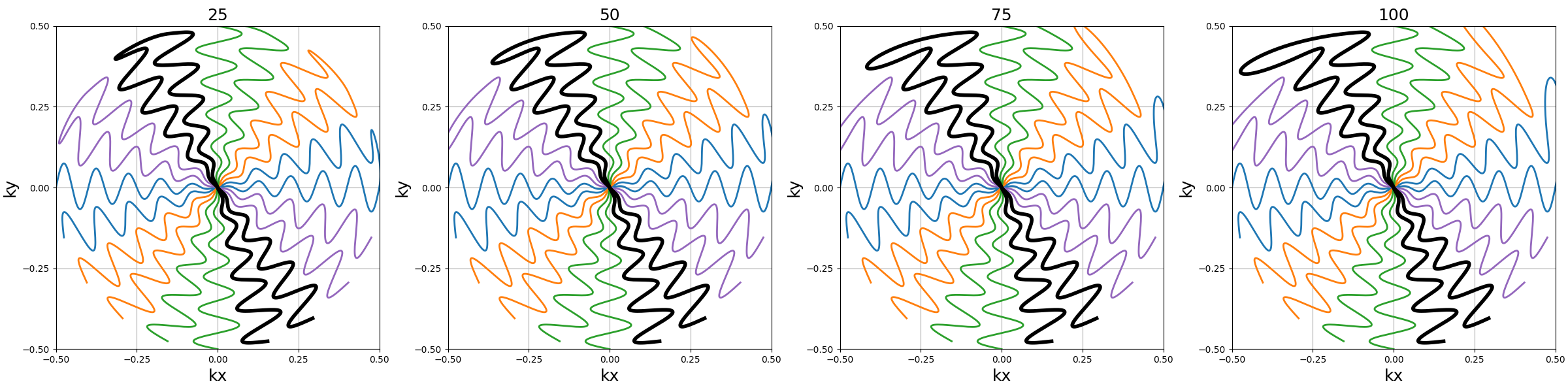
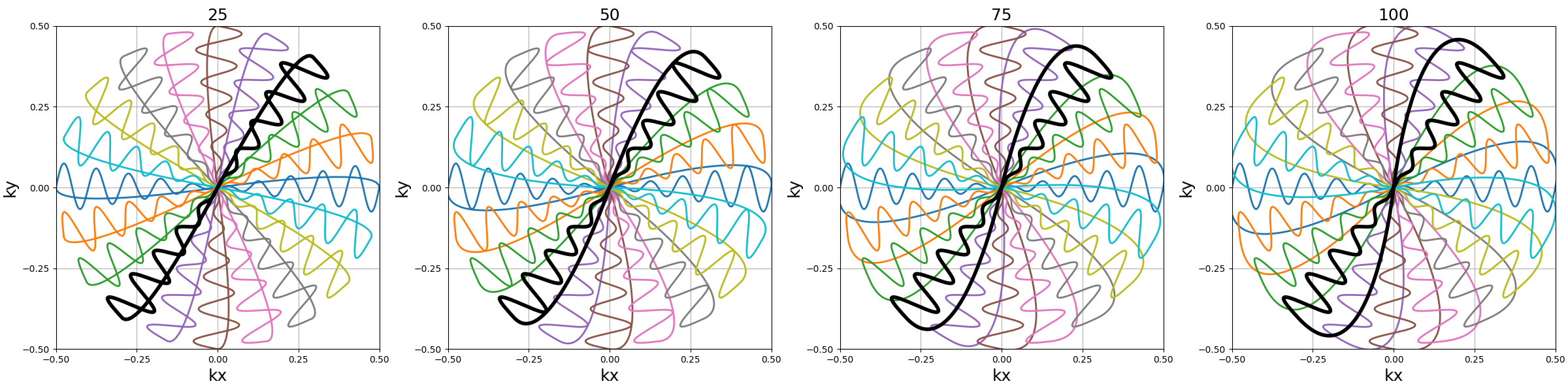
Ns_transitions (int)#
Number of samples/steps between the merged readouts. Smoother transitions are achieved with more points, but it means longer waiting times between readouts if they are split during acquisition.
arguments = [25, 50, 75, 100]
function = lambda x: tools.epify(
    planar_trajectories["2D Cones"],
    Ns_transitions=x,
    nb_trains=Nc_planes // 2,
    reverse_odd_shots=True,
)
show_trajectories(
    function, arguments, one_shot=one_shot, subfig_size=subfigure_size, dim="2D"
)
nb_trains (int)#
Number of resulting multi-readout shots, or trains.
arguments = [Nc_planes, Nc_planes // 2, Nc_planes // 4, 1]
function = lambda x: tools.epify(
    planar_trajectories["Radial"],
    Ns_transitions=50,
    nb_trains=x,
    reverse_odd_shots=True,
)
show_trajectories(
    function, arguments, one_shot=one_shot, subfig_size=subfigure_size, dim="2D"
)
reverse_odd_shots (bool)#
Whether to reverse every odd shots such that, as in most trajectories, even shots end up closer to the start of odd shots.
arguments = [True, False]
function = lambda x: tools.epify(
    planar_trajectories["Radial"],
    Ns_transitions=100,
    nb_trains=Nc_planes // 2,
    reverse_odd_shots=x,
)
show_trajectories(
    function, arguments, one_shot=one_shot, subfig_size=subfigure_size, dim="2D"
)
Prewind/rewind#
Two tools used to generate gradients before and after the trajectory.
The trajectory can be extended to start before the readout from the k-space center with null gradients and reach each shot position with the required gradient strength, and then come back to the center.
Arguments:
trajectory (array_like): trajectory to change by prolonging and merging the shots together.Ns_transitions (int): number of pre-winding/rewinding steps.
trajectory = tools.prewind(planar_trajectories["Spiral"], Ns_transitions=Ns // 10)
trajectory = tools.rewind(trajectory, Ns_transitions=Ns // 10)
show_trajectory(trajectory, figure_size=figure_size, one_shot=one_shot)
trajectory (array)#
The trajectory to change by extending them before and/or after the readouts.
Note that the radial prewinding and rewinding parts are overlapping with the actual trajectory.
arguments = ["Radial", "Spiral", "2D Cones", "3D Cones"]
function = lambda x: tools.prewind(
    tools.rewind(planar_trajectories[x], Ns_transitions=Ns // 10),
    Ns_transitions=Ns // 10,
)
show_trajectories(function, arguments, one_shot=one_shot, subfig_size=subfigure_size)
show_trajectories(
    function, arguments, one_shot=one_shot, subfig_size=subfigure_size, dim="2D"
)
Ns_transitions (int)#
Number of samples/steps before and/or after the readouts. Smoother transitions are achieved with more points, but it may imply delayed readout starts and longer TRs.
arguments = [25, 50, 75, 100]
function = lambda x: tools.prewind(
    tools.rewind(planar_trajectories["2D Cones"], Ns_transitions=x),
    Ns_transitions=x,
)
show_trajectories(
    function, arguments, one_shot=one_shot, subfig_size=subfigure_size, dim="2D"
)
Functional tools#
Preparation#
We can define a few functions that will be used in the following examples, using again 2D radial, Fermat’s spiral, and 2D/3D cones:
init_trajectories = {
    "Radial": lambda Nc: mn.initialize_2D_radial(Nc, Ns, in_out=in_out),
    "Spiral": lambda Nc: mn.initialize_2D_spiral(
        Nc, Ns, in_out=in_out, spiral="fermat", nb_revolutions=nb_revolutions
    ),
    "2D Cones": lambda Nc: mn.initialize_2D_cones(
        Nc, Ns, in_out=in_out, nb_zigzags=nb_zigzags
    ),
    "3D Cones": lambda Nc: tools.rotate(
        single_trajectories["3D Cones"],
        nb_rotations=Nc,
        z_tilt=2 * np.pi / Nc / (1 + in_out),
    ),
}
Stack spherically#
A tool similar to tools.stack but with stacks shrinked
in order to cover the k-space sphere and a variable number
of shot per stack to improve the coverage over larger stacks.
Arguments:
trajectory_func (function): trajectory function that should return an array-like with the usual \((N_c, N_s, N_d)\) size.Nc (int): number of shots to use for the whole spherically stacked trajectory.nb_stacks (int): number of stacks repeatingtrajectoryover the \(k_z\)-axis.z_tilt (float): angle tilt between consecutive stacks around the \(k_z\)-axis.(default None)hard_bounded (bool): whether the stacks should be strictly bounded to k-space.(default True)**kwargs: trajectory initialization parameters for the function provided withtrajectory_func.
trajectory = tools.stack_spherically(
    init_trajectories["Radial"], Nc=Nc, nb_stacks=nb_repetitions
)
show_trajectory(trajectory, figure_size=figure_size, one_shot=one_shot)
trajectory_func (function)#
A function that takes at least one argument Nc to control
the number of shots, in order to adapt that value for each stack
and focus more ressources over larger areas. In opposition to
tools.stack, it is not possible to use stacked-NUFFT operators
with tools.stack_spherically.
arguments = ["Radial", "Spiral", "2D Cones", "3D Cones"]
function = lambda x: tools.stack_spherically(
    init_trajectories[x], Nc=Nc, nb_stacks=nb_repetitions
)
show_trajectories(function, arguments, one_shot=one_shot, subfig_size=subfigure_size)
show_trajectories(
    function,
    arguments,
    one_shot=one_shot,
    subfig_size=subfigure_size,
    dim="2D",
    axes=(0, 2),
)
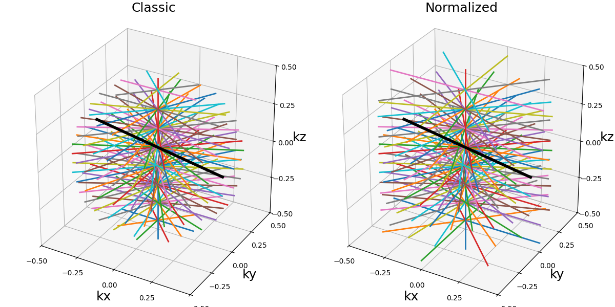
In the previous example, we can observe that spirals and cones are nicely adapted for each stack, while shrinking the shots for the radial trajectory is quite irrelevant (coverage is not improved). Instead, each radial disc could be normalized to cover a cylinder with variable density over \(k_z\).
traj_classic = tools.stack_spherically(
    init_trajectories["Radial"], Nc=Nc, nb_stacks=nb_repetitions
)
traj_normal = np.copy(traj_classic)
traj_normal[..., :2] = (
    KMAX
    * traj_normal[..., :2]
    / np.max(
        np.linalg.norm(traj_classic[..., :2], axis=2, keepdims=True),
        axis=1,
        keepdims=True,
    )
)

trajectories = {"Classic": traj_classic, "Normalized": traj_normal}
arguments = ["Classic", "Normalized"]
function = lambda x: trajectories[x]
show_trajectories(function, arguments, one_shot=one_shot, subfig_size=subfigure_size)
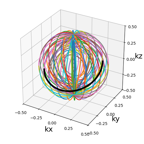
Shellify#
A tool to carve trajectories into half-spheres/domes and duplicate them into concentric shells composed of a variable number of shots depending on their size.
Arguments:
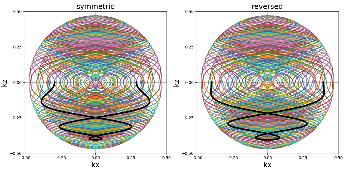
trajectory_func (function): trajectory function that should return an array-like with the usual \((N_c, N_s, N_d)\) size.Nc (int): number of shots to use for the whole spherically stacked trajectory.nb_shells (int): number of shells repeatingtrajectorywith spherical distortion over the \(k_z\)-axis.z_tilt (float): angle tilt between concentric shells around the \(k_z\)-axis.(default None)hemisphere_mode (str): define how the lower hemisphere should be oriented relatively to the upper one, with “symmetric” providing a kx-ky planar symmetry by changing the polar angle, and with “reversed” promoting continuity (for example in spirals) by reversing the azimuthal angle.(default "symmetric").**kwargs: trajectory initialization parameters for the function provided withtrajectory_func.
trajectory = tools.shellify(
    init_trajectories["Radial"], Nc=Nc, nb_shells=nb_repetitions
)
show_trajectory(trajectory, figure_size=figure_size, one_shot=one_shot)
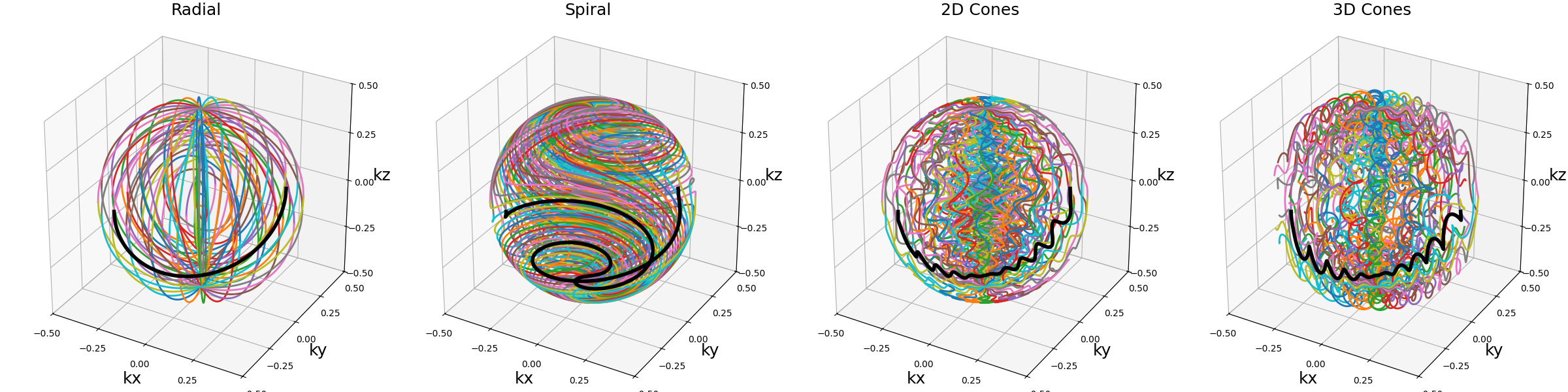
trajectory_func (function)#
A function that takes at least one argument Nc to control
the number of shots, in order to adapt that value for each shell
and focus more ressources over larger spheres.
Gradient amplitudes and slew rates are likely to be increased near the edges, and it should be accounted for. Companion functions will be added in the future in order to manipulate individual spheres.
arguments = ["Radial", "Spiral", "2D Cones", "3D Cones"]
function = lambda x: tools.shellify(
    init_trajectories[x], Nc=Nc, nb_shells=nb_repetitions
)
show_trajectories(function, arguments, one_shot=one_shot, subfig_size=subfigure_size)
hemisphere_mode (str)#
Define how the lower hemisphere should be oriented relatively to the upper one, with “symmetric” providing a \(k_x-k_y\) planar symmetry by changing the polar angle, and with “reversed” promoting continuity (for example in spirals) by reversing the azimuthal angle.
arguments = ["symmetric", "reversed"]
function = lambda x: tools.shellify(
    init_trajectories["Spiral"], Nc=Nc, nb_shells=nb_repetitions, hemisphere_mode=x
)
show_trajectories(
    function,
    arguments,
    one_shot=one_shot,
    subfig_size=subfigure_size,
    dim="2D",
    axes=(0, 2),
)
References#
Pipe, James G., Nicholas R. Zwart, Eric A. Aboussouan, Ryan K. Robison, Ajit Devaraj, and Kenneth O. Johnson. “A new design and rationale for 3D orthogonally oversampled k‐space trajectories.” Magnetic resonance in medicine 66, no. 5 (2011): 1303-1311.
Total running time of the script: (1 minutes 14.843 seconds)