3D Trajectories

A collection of 3D non-Cartesian trajectories with analytical definitions.

Hereafter we detail and illustrate the different arguments used in the parameterization of 3D non-Cartesian trajectories. Since most arguments are redundant across the different patterns, some of the documentation will refer to previous patterns for explanation.

Note that the examples hereafter only cover natively 3D trajectories or famous 3D trajectories obtained from 2D. Examples on how to use tools to make 3D trajectories out of 2D ones are presented in Trajectory tools

In this page in particular, we invite the user to manually run the script to be able to manipulate the plot orientations with the matplotlib interface to better visualize the 3D volumes.

# External
import matplotlib.pyplot as plt
import numpy as np
from utils import show_trajectories, show_trajectory

# Internal
import mrinufft as mn
from mrinufft import display_2D_trajectory, display_3D_trajectory

Script options

These options are used in the examples below as default values for all trajectories.

# Trajectory parameters
Nc = 120  # Number of shots
Ns = 500  # Number of samples per shot
in_out = False  # Choose between in-out or center-out trajectories
tilt = "uniform"  # Angular distance between shots
nb_repetitions = 6  # Number of stacks, rotations, cones, shells etc.
nb_revolutions = 1  # Number of revolutions for base trajectories

# Display parameters
figure_size = 10  # Figure size for trajectory plots
subfigure_size = 6  # Figure size for subplots
one_shot = -5  # Highlight one shot in particular

Radial trajectories

In this section are presented trajectories based on radial lines oriented using different methods and structures.

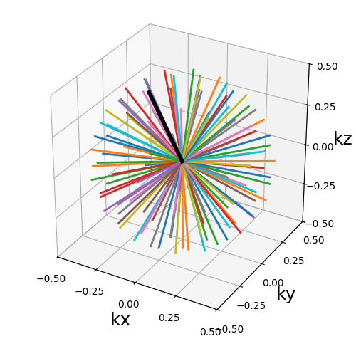
Phyllotaxis radial

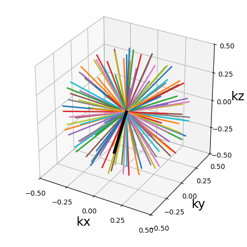
A 3D radial pattern with phyllotactic structure.

The radial shots are oriented according to a Fibonacci sphere lattice, supposed to reproduce the phyllotaxis found in nature through flowers, etc. It ensures an almost uniform distribution.

This function reproduces the proposition from [Pic+11], but the name “spiral phyllotaxis” was changed to avoid confusion with actual spirals.

Arguments:

• Nc (int): number of individual shots

• Ns (int): number of samples per shot

• in_out (bool): define whether the shots should travel toward the center then outside (in-out) or not (center-out). (default False)

trajectory = mn.initialize_3D_phyllotaxis_radial(Nc, Ns, in_out=in_out)
show_trajectory(trajectory, figure_size=figure_size, one_shot=one_shot)

Nc (int)

The number of individual shots, here 3D radial lines, used to cover the k-space. More shots means better coverage but also longer acquisitions.

arguments = [Nc // 4, Nc // 2, Nc, Nc * 2]
function = lambda x: mn.initialize_3D_phyllotaxis_radial(x, Ns, in_out=in_out)
show_trajectories(function, arguments, one_shot=one_shot, subfig_size=subfigure_size)

Ns (int)

The number of samples per shot. More samples means that either the acquisition window is lengthened or the sampling rate is increased.

arguments = [10, 25, 40, 100]
function = lambda x: mn.initialize_3D_phyllotaxis_radial(Nc, x, in_out=in_out)
show_trajectories(function, arguments, one_shot=one_shot, subfig_size=subfigure_size)

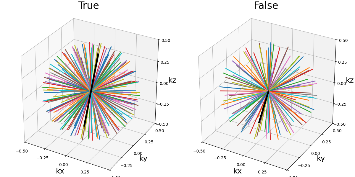
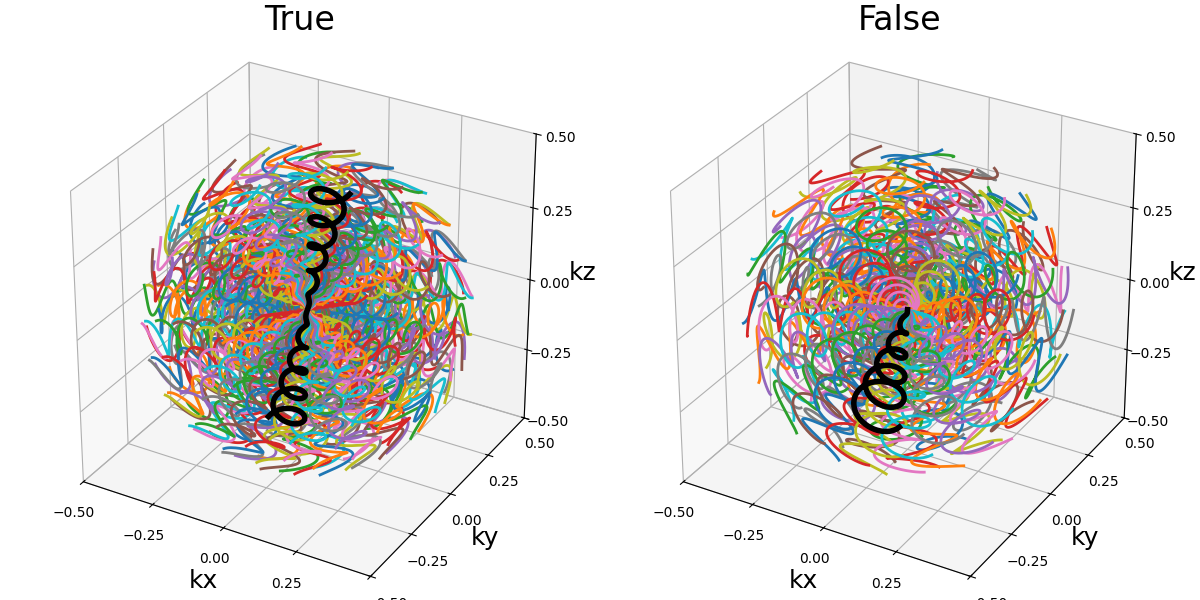
in_out (bool)

It allows switching between different ways to define how the shot should travel through the k-space:

• in-out: starting from the outer regions, then passing through the center then going back to outer regions, often on the opposite side (radial, cones)

• center-out or center-center: when in_out=False the trajectory will start at the center, but depending on the specific trajectory formula the path might end up in the outer regions (radial, spiral, cones, etc) or back to the center (rosette, lissajous).

Note that the behavior of both tilt and width are automatically adapted to the changes to avoid having to update them too when switching in_out.

arguments = [True, False]
function = lambda x: mn.initialize_3D_phyllotaxis_radial(Nc, Ns, in_out=x)
show_trajectories(function, arguments, one_shot=one_shot, subfig_size=subfigure_size)

Golden means radial

A 3D radial pattern with golden means-based structure.

The radial shots are oriented using multidimensional golden means, which are derived from modified Fibonacci sequences by an eigenvalue approach, to provide a temporally stable acquisition with widely spread shots at all time.

This function reproduces the proposition from [Cha+09], with in addition the option to switch between center-out and in-out radial shots.

Arguments:

• Nc (int): number of individual shots. See 3D radial

• Ns (int): number of samples per shot. See 3D radial

• in_out (bool): define whether the shots should travel toward the center then outside (in-out) or not (center-out). (default False). See 3D radial

trajectory = mn.initialize_3D_golden_means_radial(Nc, Ns, in_out=in_out)
show_trajectory(trajectory, figure_size=figure_size, one_shot=one_shot)

Wong radial

A 3D radial pattern with a spiral structure.

The radial shots are oriented according to an archimedean spiral over a sphere surface, for each interleave.

This function reproduces the proposition from [WR94], with in addition the option to switch between center-out and in-out radial shots.

Arguments:

• Nc (int): number of individual shots. See 3D radial

• Ns (int): number of samples per shot. See 3D radial

• nb_interleaves (int): number of implicit interleaves defining the shots order for a more structured k-space distribution over time. (default 1)

• in_out (bool): define whether the shots should travel toward the center then outside (in-out) or not (center-out). (default False). See 3D radial

trajectory = mn.initialize_3D_wong_radial(Nc, Ns, in_out=in_out)
show_trajectory(trajectory, figure_size=figure_size, one_shot=one_shot)

Park radial

A 3D radial pattern with a spiral structure.

The radial shots are oriented according to an archimedean spiral over a sphere surface, shared uniformly between all interleaves.

This function reproduces the proposition from [Par+16], itself based on the work from [WR94], with in addition the option to switch between center-out and in-out radial shots.

Arguments:

• Nc (int): number of individual shots. See 3D radial

• Ns (int): number of samples per shot. See 3D radial

• nb_interleaves (int): number of implicit interleaves defining the shots order for a more structured k-space distribution over time. (default 1)

• in_out (bool): define whether the shots should travel toward the center then outside (in-out) or not (center-out). (default False). See 3D radial

trajectory = mn.initialize_3D_park_radial(Nc, Ns, in_out=in_out)
show_trajectory(trajectory, figure_size=figure_size, one_shot=one_shot)

Freeform trajectories

In this section are presented trajectories in all kinds of shapes and relying on different principles.

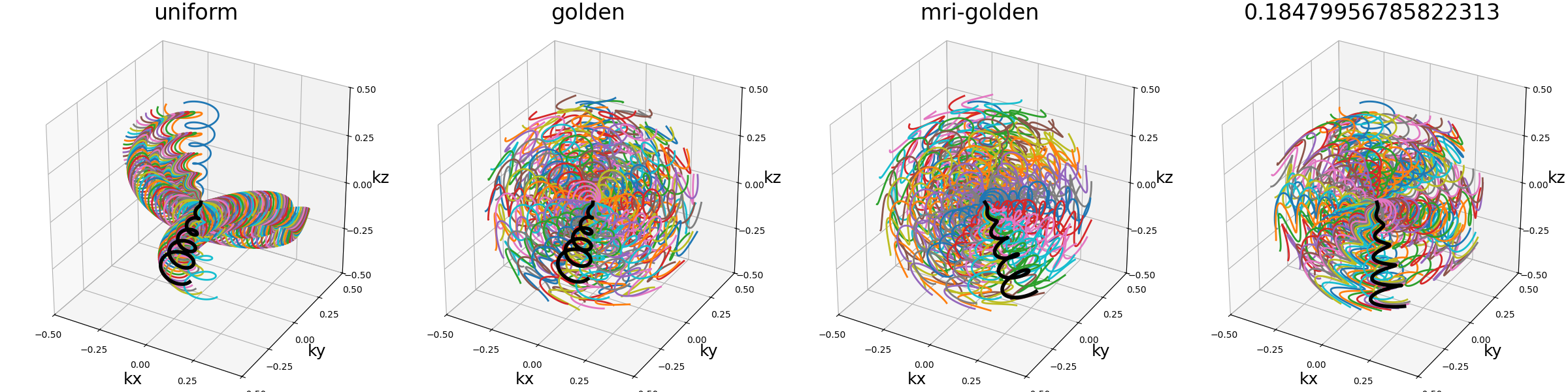
3D Cones

A common pattern composed of 3D cones oriented all over within a sphere.

Arguments:

• Nc (int): number of individual shots. See 3D radial

• Ns (int): number of samples per shot. See 3D radial

• tilt (str, float): angle between each consecutive shot (in radians). (default "golden")

• in_out (bool): define whether the shots should travel toward the center then outside (in-out) or not (center-out). (default False). See 3D radial

• nb_zigzags (float): number of revolutions over a center-out shot. (default 5)

• spiral (str, float): type of spiral defined through the general archimedean equation. (default "archimedes"). See 2D spiral

• width (float): cone width factor, normalized to densely cover the k-space by default. (default 1)

trajectory = mn.initialize_3D_cones(Nc, Ns, in_out=in_out)
show_trajectory(trajectory, figure_size=figure_size, one_shot=one_shot)

tilt (str, float)

The angle between each consecutive shots, either in radians or as a string defining some default mods such as “uniform” for \(2 \pi / N_c\), or “golden” and “mri golden” for the different common definitions of golden angles. The angle is automatically adapted when the in_out argument is switched to keep the same behavior.

arguments = ["uniform", "golden", "mri-golden", np.pi / 17]
function = lambda x: mn.initialize_3D_cones(Nc, Ns, tilt=x, in_out=in_out)
show_trajectories(function, arguments, one_shot=one_shot, subfig_size=subfigure_size)

nb_zigzags (float)

The number of “zigzags”, or revolutions around the 3D cone on a center-out shot (doubled overall for in-out trajectories)

arguments = [0.5, 2, 5, 10]
function = lambda x: mn.initialize_3D_cones(Nc, Ns, in_out=in_out, nb_zigzags=x)
show_trajectories(function, arguments, one_shot=one_shot, subfig_size=subfigure_size)

spiral (str, float)

The shape of the spiral defined and documented in initialize_2D_spiral. Both "archimedes" and "fermat" spirals are available as string options for convenience.

arguments = ["archimedes", "fermat", 0.5, 1.5]
function = lambda x: mn.initialize_3D_cones(Nc, Ns, in_out=in_out, spiral=x)
show_trajectories(function, arguments, one_shot=one_shot, subfig_size=subfigure_size)

width (float)

The cone width normalized such that width = 1 corresponds to non-overlapping cones covering the whole k-space sphere, and therefore width > 1 creates overlap between cone regions and width < 1 tends to more radial patterns.

arguments = [0.2, 1, 2, 3]
function = lambda x: mn.initialize_3D_cones(Nc, Ns, in_out=in_out, width=x)
show_trajectories(function, arguments, one_shot=one_shot, subfig_size=subfigure_size)

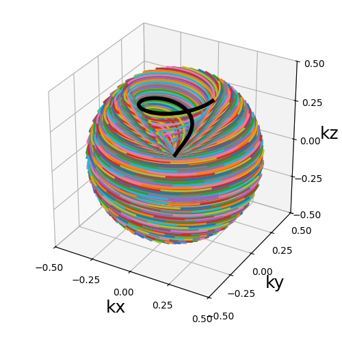
FLORET

A pattern introduced in [Pip+11] composed of Fermat spirals folded into cones. The acronym stands for Fermat Looped, Orthogonally Encoded Trajectories. Most arguments are related either to initialize_2D_spiral or to tools.conify.

Arguments:

• Nc (int): number of individual shots. See 3D radial

• Ns (int): number of samples per shot. See 3D radial

• in_out (bool): define whether the shots should travel toward the center then outside (in-out) or not (center-out). (default False). See 3D radial

• nb_revolutions (float): number of revolutions performed from the center. (default 1). See 2D spiral

• spiral (str, float): type of spiral defined through the general archimedean equation. (default "fermat"). See 2D spiral

• cone_tilt (float): angle tilt between consecutive cones around the \(k_z\)-axis. (default "golden"). See tools.conify

• max_angle (float): maximum angle of the cones. (default pi / 2). See tools.conify

• axes (tuple): axes over which cones are created, by default (2,)

trajectory = mn.initialize_3D_floret(
    Nc * nb_repetitions,
    Ns,
    in_out=in_out,
    nb_revolutions=nb_revolutions,
    max_angle=np.pi / 3,
)[::-1]
show_trajectory(trajectory, figure_size=figure_size, one_shot=one_shot)

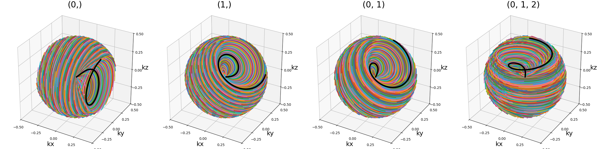
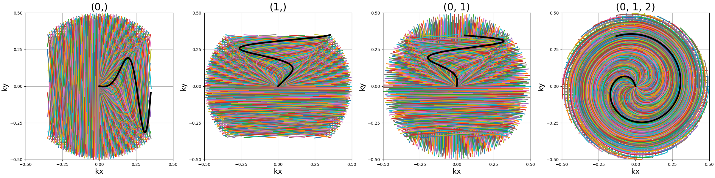
axes (tuple)

Indices of the different axes over which cones are created, with 0, 1, 2 corresponding to \(k_x, k_y, k_z\) respectively. The Nc shots and nb_cones are distributed over all axes, and therefore should be divisible by len(axes).

The point is to provide an efficient coverage by reducing max_angle to avoid redundancy around one axis, but still cover the whole k-space sphere by duplicating cones along several axes, as initially proposed by [Pip+11].

arguments = [(0,), (1,), (0, 1), (0, 1, 2)]
function = lambda x: mn.initialize_3D_floret(
    Nc * nb_repetitions,
    Ns,
    in_out=in_out,
    nb_revolutions=nb_revolutions,
    max_angle=np.pi / 4,
    axes=x,
)[::-1]
show_trajectories(function, arguments, one_shot=one_shot, subfig_size=subfigure_size)

show_trajectories(
    function, arguments, one_shot=one_shot, subfig_size=subfigure_size, dim="2D"
)

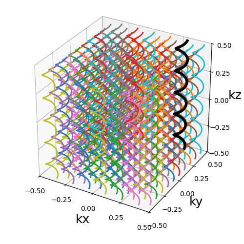
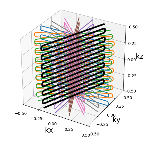
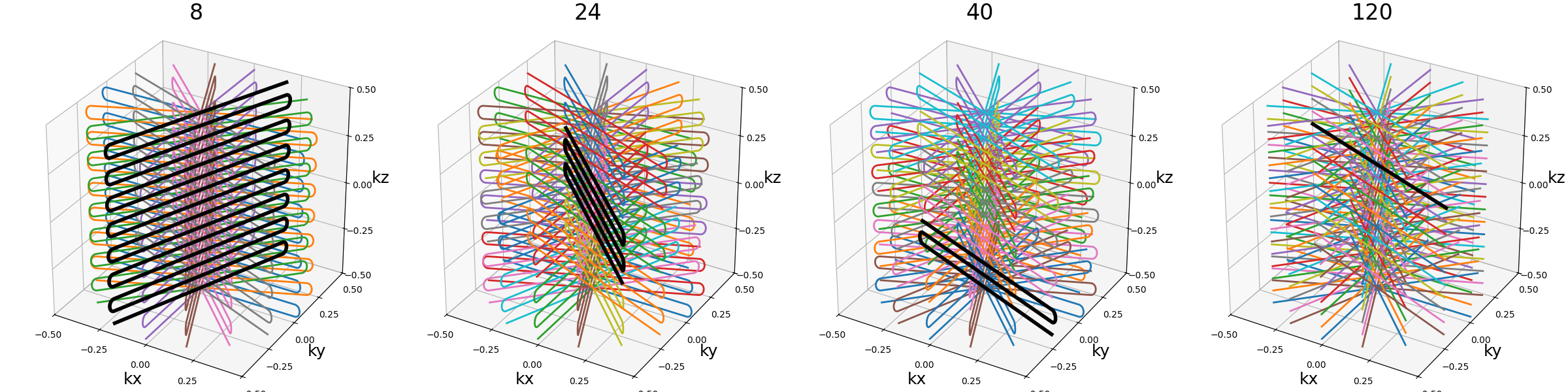
Wave-CAIPI

A pattern introduced in [Bil+15] composed of helices evolving in the same direction and packed together, inherited from trajectories such as CAIPIRINHA and Bunched Phase-Encoding (BPE) designed to better spread aliasing and facilitate reconstruction.

Arguments:

• Nc (int): number of individual shots. See 3D radial

• Ns (int): number of samples per shot. See 3D radial

• nb_revolutions (str, float): number of revolution of the helices. (default 5)

• width (float): helix width factor, normalized to densely cover the k-space by default. (default 1).

• packing (str): packing method used to position the helices. (default "triangular")

• shape (str, float): shape over the 2D kx-ky plane to pack with shots. (default "circle")

• spacing (tuple(int, int)): Spacing between helices over the 2D \(k_x\)-\(k_y\) plane normalized similarly to width. (default (1, 1))

trajectory = mn.initialize_3D_wave_caipi(Nc, Ns)
show_trajectory(trajectory, figure_size=figure_size, one_shot=one_shot)

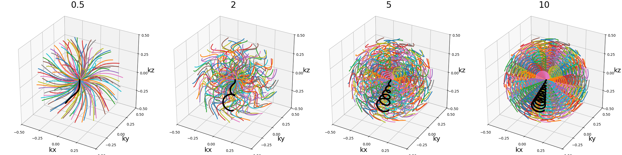
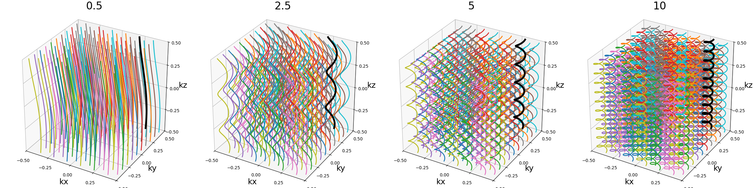
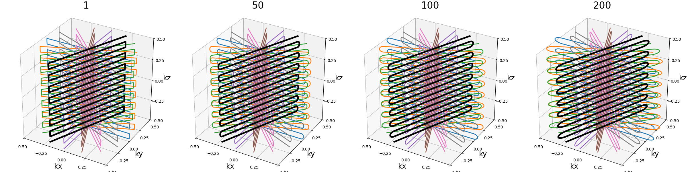
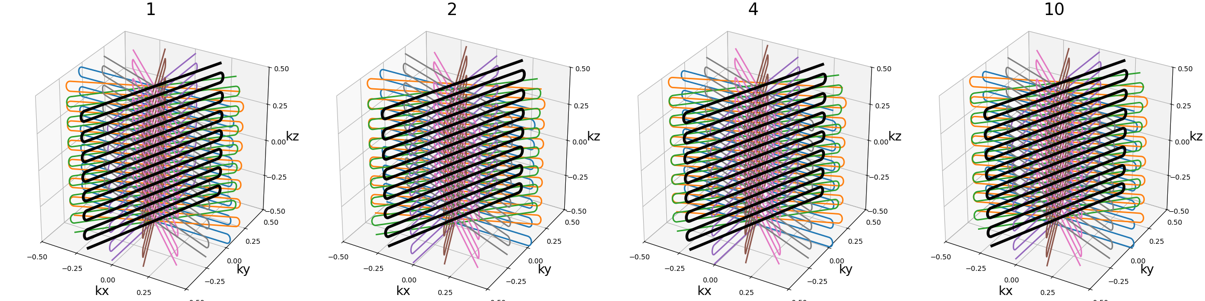
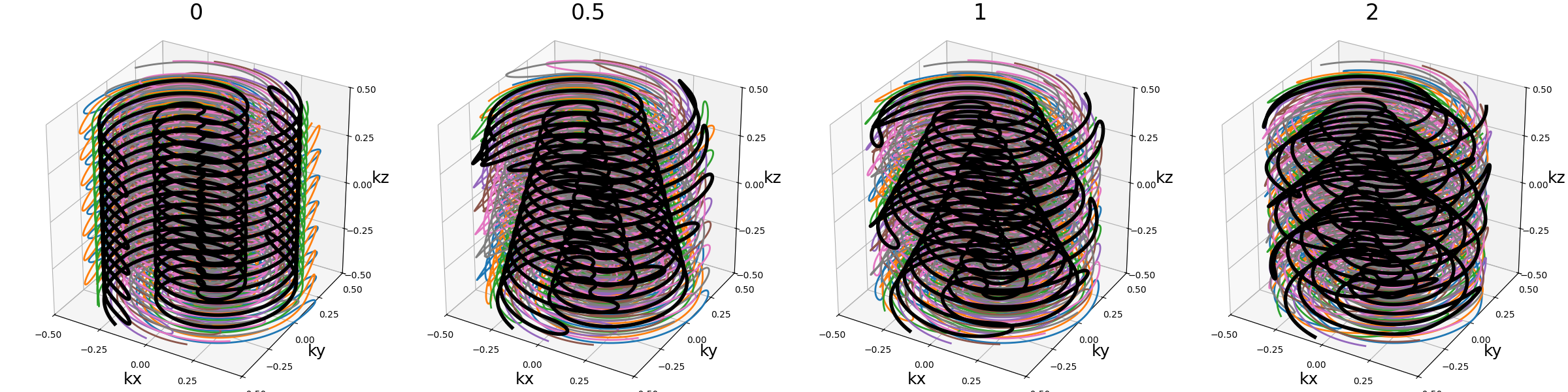
nb_revolutions (float)

The number of revolutions of the helices from bottom to top.

arguments = [0.5, 2.5, 5, 10]
function = lambda x: mn.initialize_3D_wave_caipi(Nc, Ns, nb_revolutions=x)
show_trajectories(function, arguments, one_shot=one_shot, subfig_size=subfigure_size)

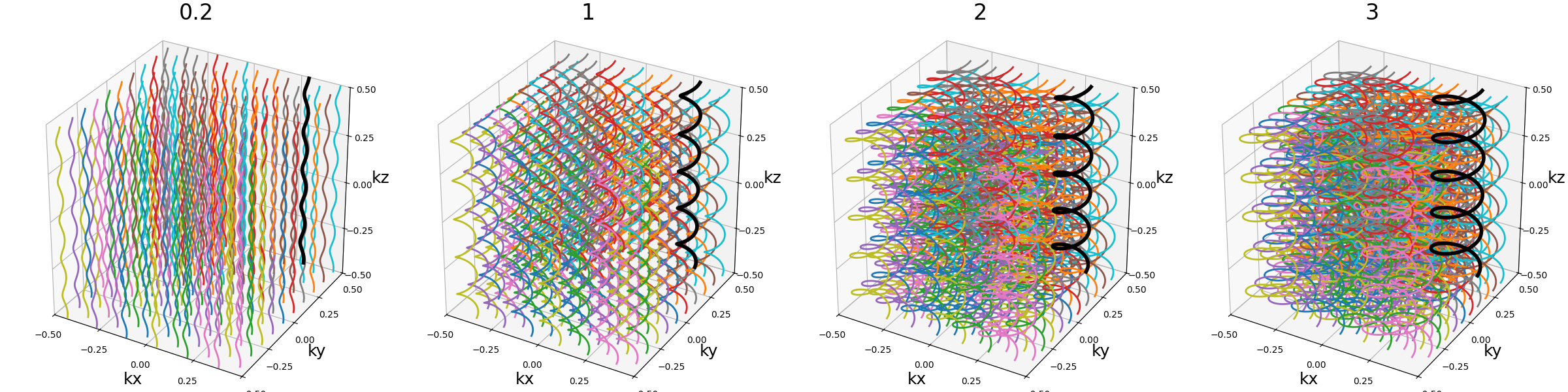
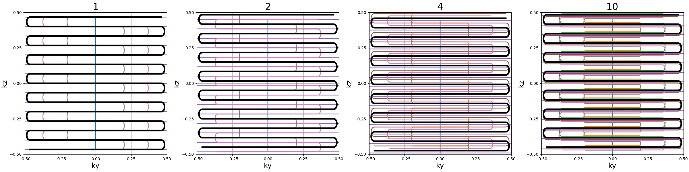
width (float)

The helix diameter normalized such that width = 1 corresponds to non-overlapping shots densely covering the k-space shape (for square packing), and therefore width > 1 creates overlap between cone regions and width < 1 tends to more radial patterns.

See packing for more details about coverage.

arguments = [0.2, 1, 2, 3]
function = lambda x: mn.initialize_3D_wave_caipi(Nc, Ns, width=x)
show_trajectories(function, arguments, one_shot=one_shot, subfig_size=subfigure_size)

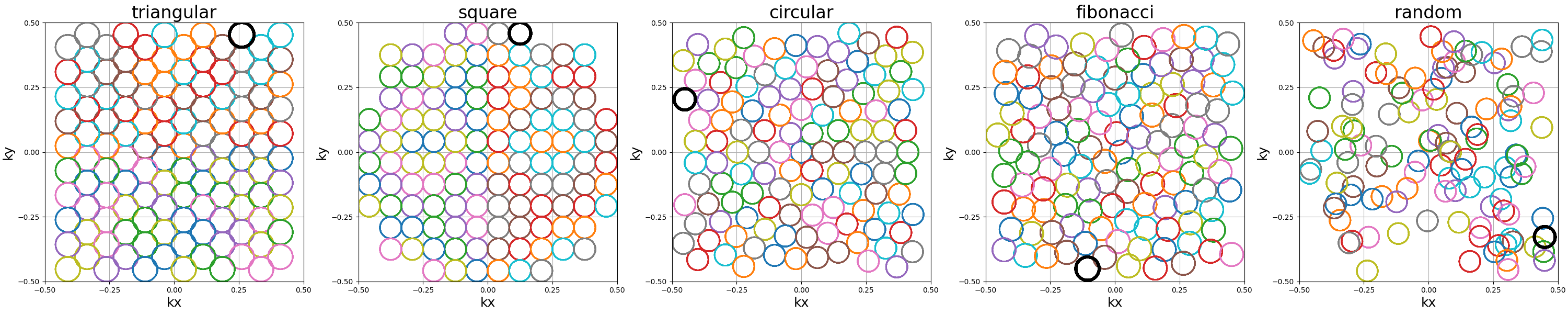
packing (str)

The method used to pack circles of same size within an arbitrary shape. The available methods are "triangular" and "square" for regular tiling over dense grids, and "circular", fibonacci and "random" for irregular packing. Different aliases are available, such as "triangle", "hexagon" instead of "triangular".

Note that "triangular" and fibonacci packings have slightly overlapping helices, as their widths correspond to that of an optimaly packed triangular/hexagonal grid. The "random" packing also naturally overlaps as the positions are determined following a uniform distribution over \(k_x\) and \(k_y\) dimensions.

arguments = ["triangular", "square", "circular", "fibonacci", "random"]
function = lambda x: mn.initialize_3D_wave_caipi(Nc, Ns, packing=x)
show_trajectories(function, arguments, one_shot=one_shot, subfig_size=subfigure_size)

show_trajectories(
    function, arguments, one_shot=one_shot, subfig_size=subfigure_size, dim="2D"
)

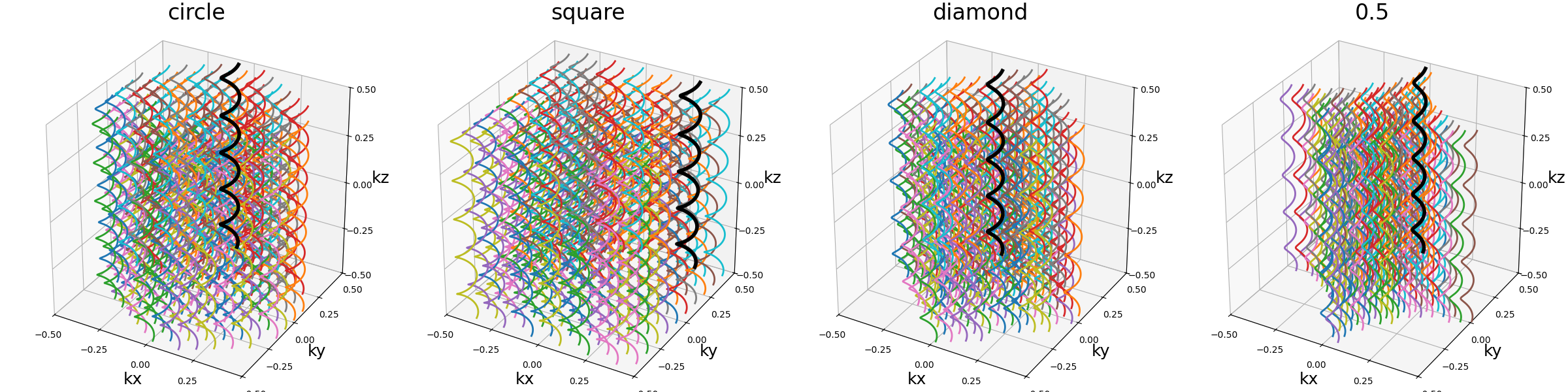
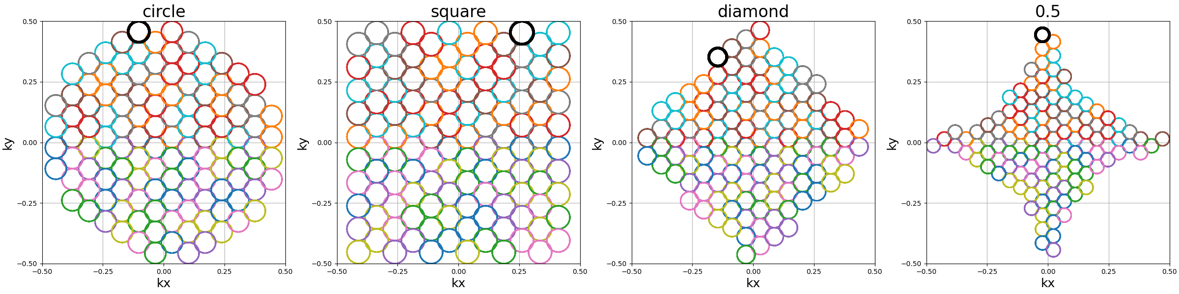
shape (str, float)

The 2D shape defined over the \(k_x\)-\(k_y\) plane and where the helices should be packed. Aliases are available for convenience, namely "circle", "square", "diamond", but shapes are primarily defined through the p-norm of the 2D coordinates following the convention of the ord parameter from numpy.linalg.norm.

The shapes are approximately respected depending on the available Nc parameter, and extra shots on the edges will be placed in priority to have a minimal 2-norm (eliminating the diagonals) except for circles with infinity-norm (accumulating over the diagonals).

arguments = ["circle", "square", "diamond", 0.5]
function = lambda x: mn.initialize_3D_wave_caipi(Nc, Ns, shape=x)
show_trajectories(function, arguments, one_shot=one_shot, subfig_size=subfigure_size)

show_trajectories(
    function, arguments, one_shot=one_shot, subfig_size=subfigure_size, dim="2D"
)

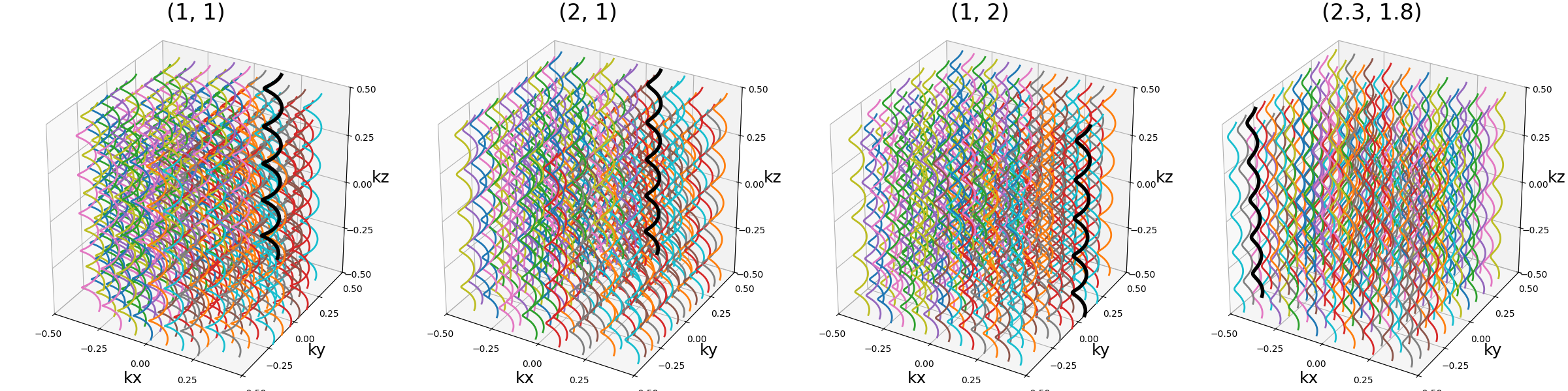
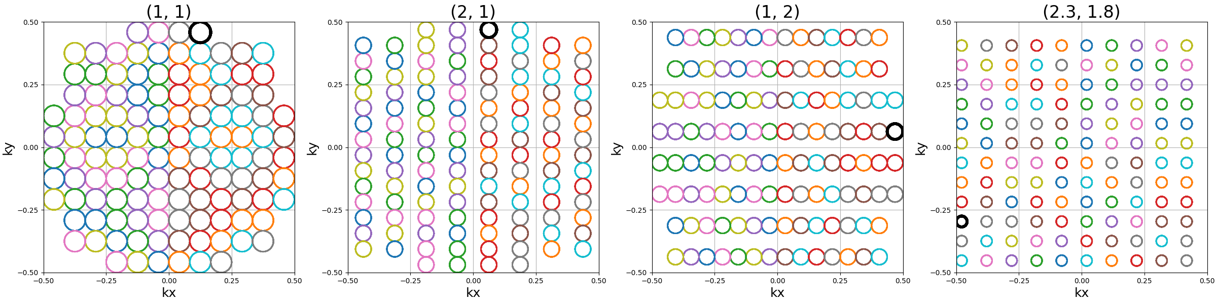
spacing (tuple(int, int))

The spacing between helices over the \(k_x\)-\(k_y\) plane, mostly defined for "square" packing. It is defined to correspond to the width unit, itself automatically matching the helix diameters, which can cause more complex behaviors for other packing methods as the diameters are normalized to fit within the cubic k-space.

arguments = [(1, 1), (2, 1), (1, 2), (2.3, 1.8)]
function = lambda x: mn.initialize_3D_wave_caipi(Nc, Ns, packing="square", spacing=x)
show_trajectories(function, arguments, one_shot=one_shot, subfig_size=subfigure_size)

show_trajectories(
    function, arguments, one_shot=one_shot, subfig_size=subfigure_size, dim="2D"
)

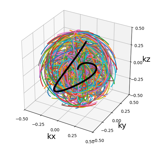
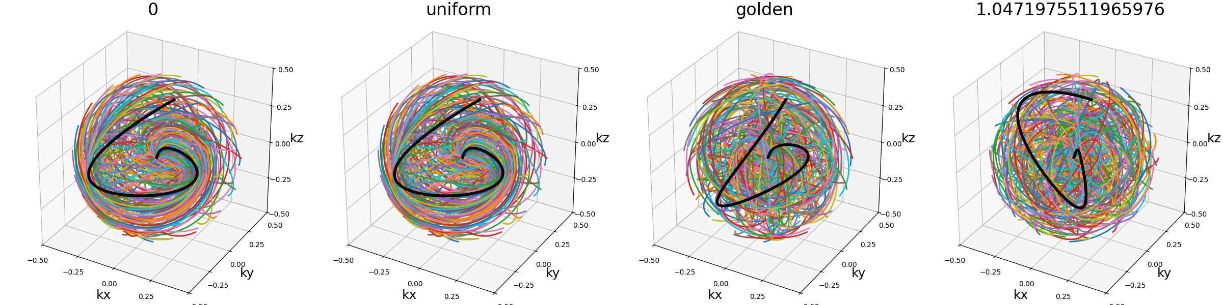
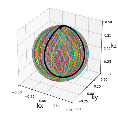
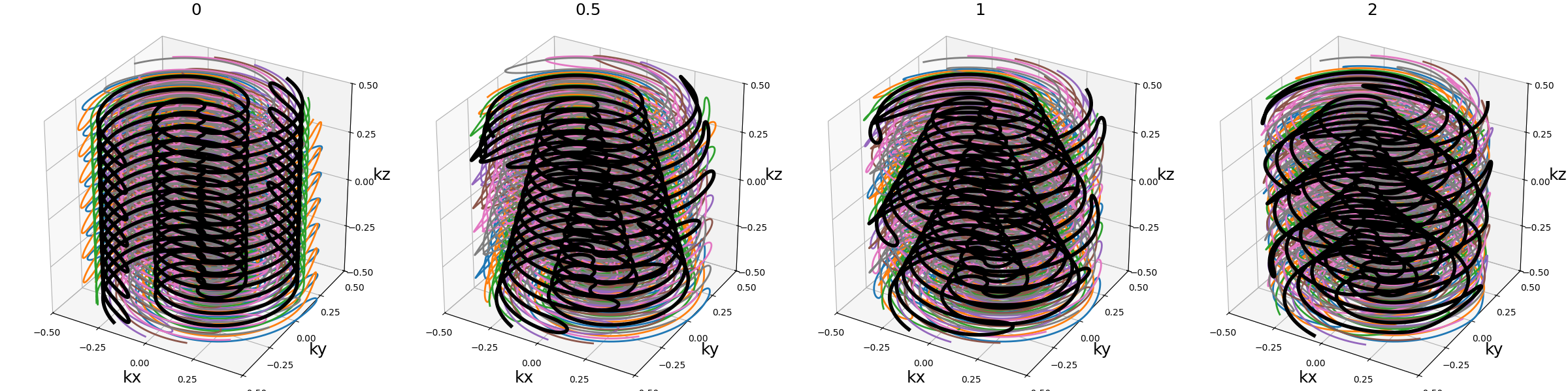
Seiffert spirals / Yarnball

A recent pattern with tightly controlled gradient norms using radially modulated Seiffert spirals, based on Jacobi elliptic functions. Note that Seiffert spirals more commonly refer to a curve evolving over a sphere surface rather than a volume, with the advantage of having a constant speed and angular velocity. The MR trajectory is obtained by increasing progressively the radius of the sphere.

This implementation follows the proposition from [SMR18] based on works from [Er00] and [Br09]. The pattern is also referred to as Yarnball by a different team [SB21], as a nod to the Yarn trajectory pictured in [IN95], even though both admittedly share little in common.

Arguments:

• Nc (int): number of individual shots. See 3D radial

• Ns (int): number of samples per shot. See 3D radial

• curve_index (float): Index controlling curvature from 0 (flat) to 1 (curvy). (default 0.3)

• nb_revolutions (float): number of revolutions or elliptic periods. (default 1)

• axis_tilt (str, float): angle between each consecutive shot (in radians) while descending over the \(k_z\)-axis (default "golden"). See 3D cones

• spiral_tilt (str, float): angle of the spiral within its own axis, defined from center to its outermost point (default "golden").

• in_out (bool): define whether the shots should travel toward the center then outside (in-out) or not (center-out). (default False). See 3D radial

trajectory = mn.initialize_3D_seiffert_spiral(Nc, Ns, in_out=in_out)
show_trajectory(trajectory, figure_size=figure_size, one_shot=one_shot)

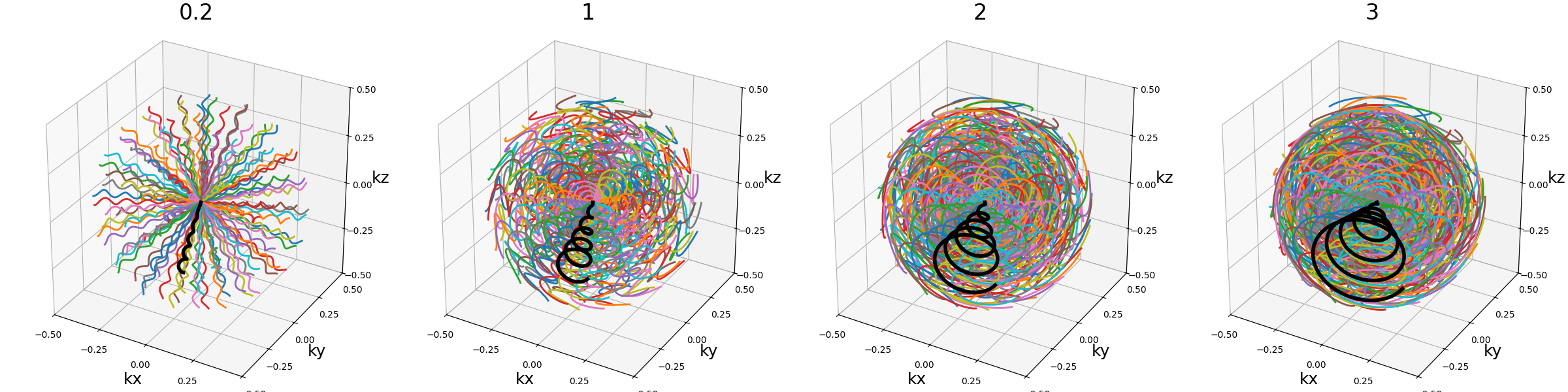
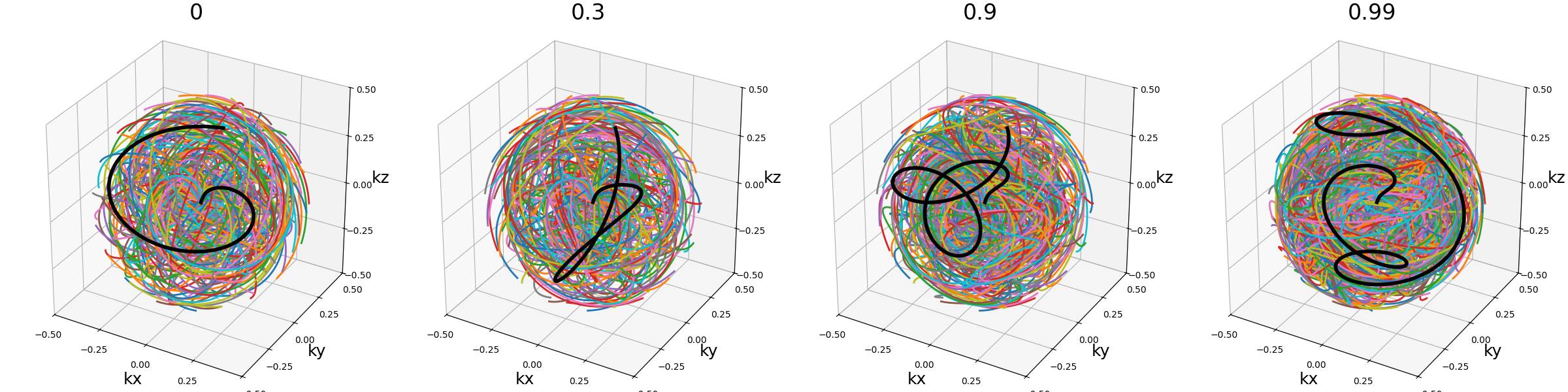
curve_index (float)

An index defined over \([0, 1)\) controling the curvature, with \(0\) corresponding to a planar spiral, and increasing the length and exploration of the curve while asymptotically approaching \(1\).

arguments = [0, 0.3, 0.9, 0.99]
function = lambda x: mn.initialize_3D_seiffert_spiral(
    Nc, Ns, in_out=in_out, curve_index=x
)
show_trajectories(function, arguments, one_shot=one_shot, subfig_size=subfigure_size)

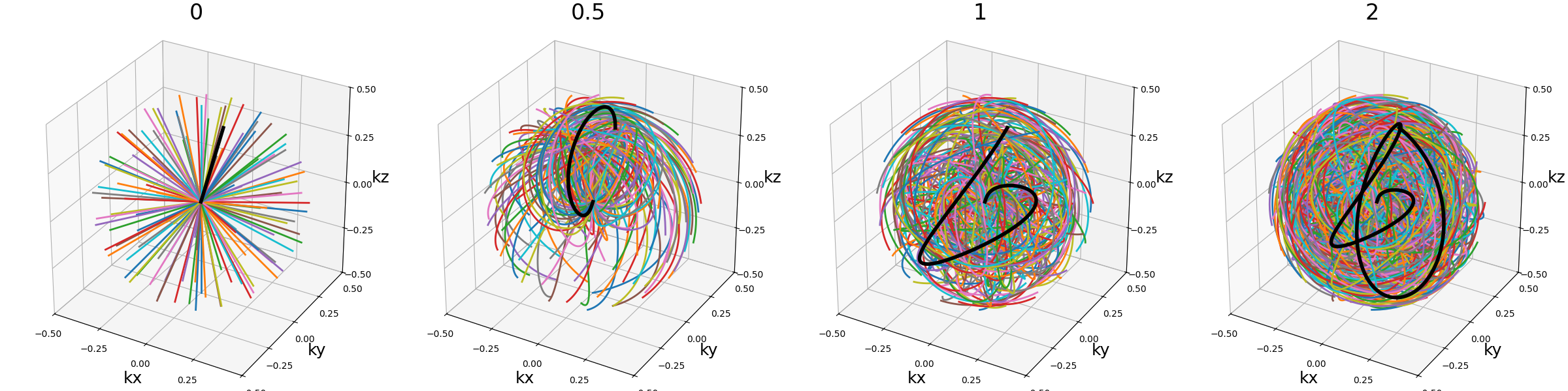
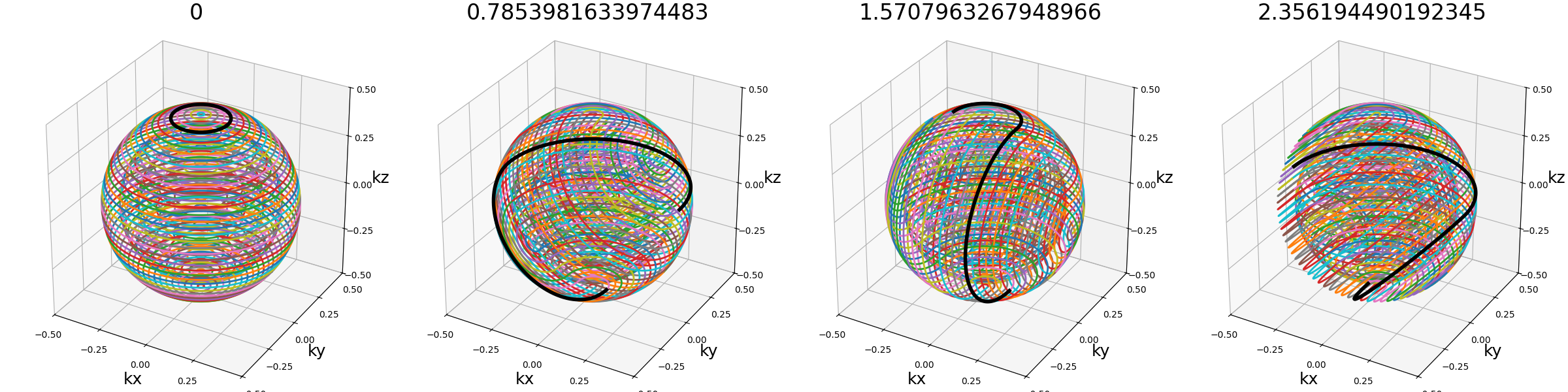
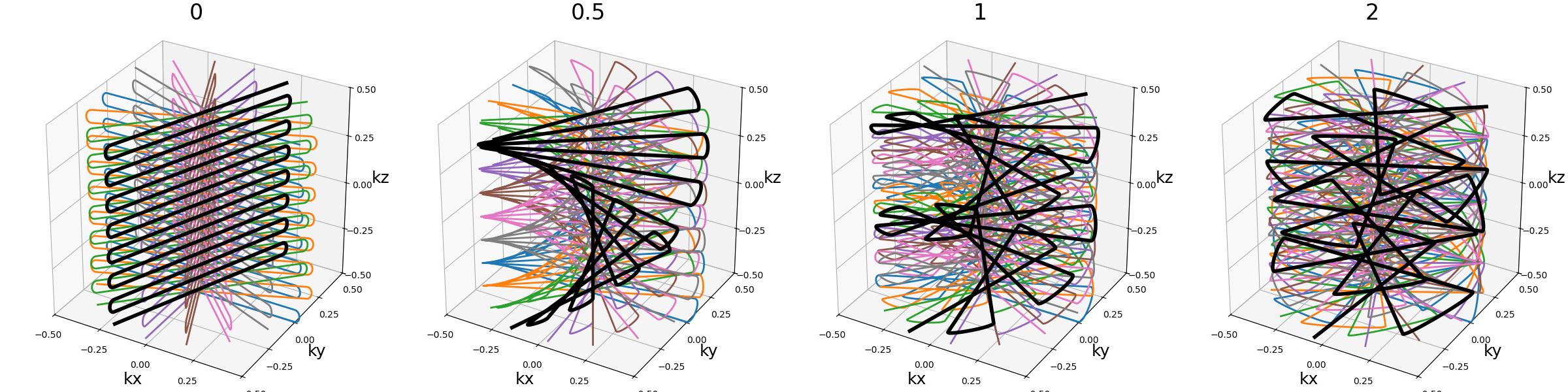
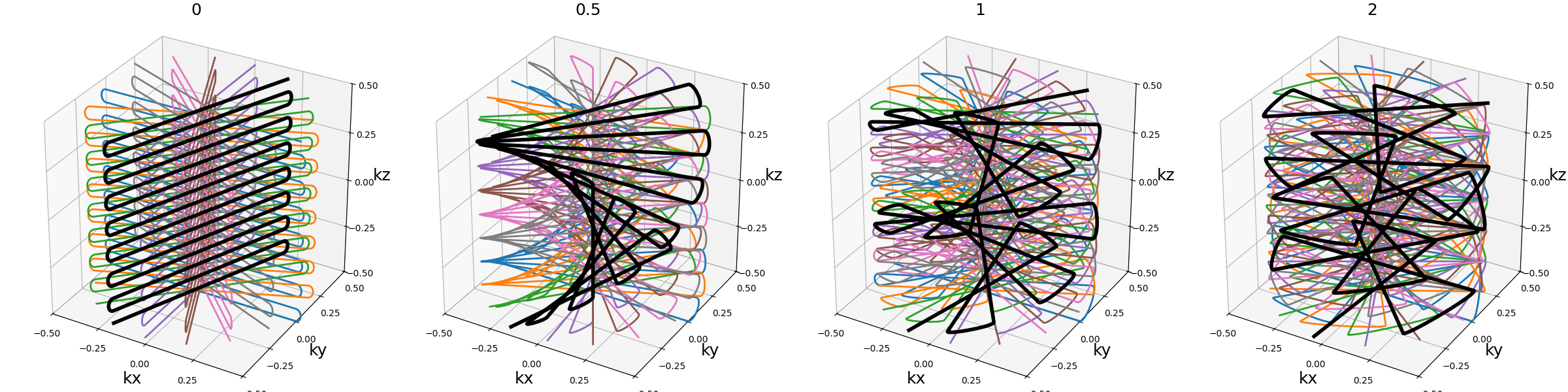
nb_revolutions (float)

Number of revolutions, or simply the number of times a curve reaches its original orientation. For regular Seiffert spirals, it corresponds to the number of times the shot reaches the starting pole of the sphere. It subsequently defines the length of the curve.

arguments = [0, 0.5, 1, 2]
function = lambda x: mn.initialize_3D_seiffert_spiral(
    Nc,
    Ns,
    in_out=in_out,
    nb_revolutions=x,
)
show_trajectories(function, arguments, one_shot=one_shot, subfig_size=subfigure_size)

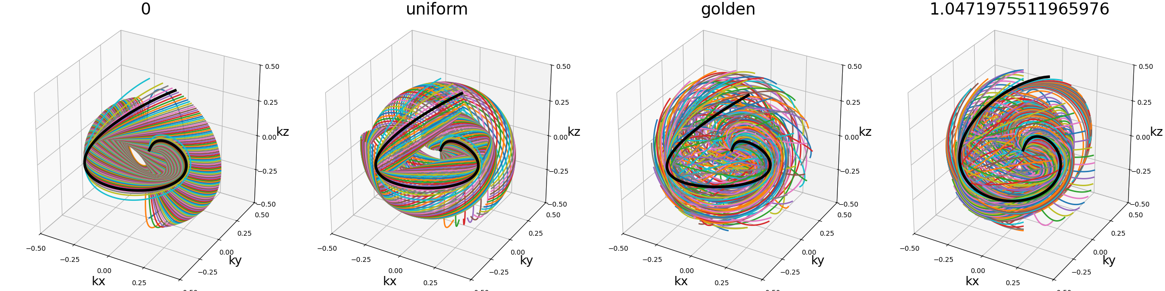
axis_tilt (str, float)

Angle between consecutive shots while descending along the \(k_z\)-axis. The "golden" value chosen as default provides an almost even distribution over the k-space sphere by relying on Fibonacci lattice, and therefore it should be changed carefully when relevant.

Note that in the examples below, the spiral_tilt argument is set to 0 for clarity.

arguments = [0, "uniform", "golden", 20 * 2 * np.pi / Nc]
function = lambda x: mn.initialize_3D_seiffert_spiral(
    Nc,
    Ns,
    in_out=in_out,
    axis_tilt=x,
    spiral_tilt=0,
)
show_trajectories(function, arguments, one_shot=one_shot, subfig_size=subfigure_size)

spiral_tilt (str, float)

Define the angle of the spiral within its own axis after precession of the spiral along the \(k_z\)-axis. Since the precession is applied through Rodrigues’ coefficients and Seiffert spirals are asymetric, their orientation right after the precession can be quite biased and yield unbalanced densities.

The method proposed in [SMR18] to handle that issue is to rotate the spirals along their own axes, but the exact way to choose the rotation is not specified. Rather than picking random angles, we decided to provide the conventional “tilt” argument.

arguments = [0, "uniform", "golden", 20 * 2 * np.pi / Nc]
function = lambda x: mn.initialize_3D_seiffert_spiral(
    Nc,
    Ns,
    in_out=in_out,
    axis_tilt="golden",
    spiral_tilt=x,
)
show_trajectories(function, arguments, one_shot=one_shot, subfig_size=subfigure_size)

Shell trajectories

In this section are presented trajectories that are composed of concentric shells, i.e. shots arranged over spherical surfaces.

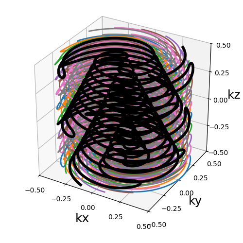
Helical shells

An arrangement of spirals covering sphere surfaces, often referred to as concentric shells. Here the name was changed to avoid confusion with other trajectories sharing this principle.

This implementation follows the proposition from [YRB06] but the idea is much older and can be traced back at least to [IN95].

Arguments:

• Nc (int): number of individual shots. See 3D radial

• Ns (int): number of samples per shot. See 3D radial

• nb_shells (int): number of shells used to partition the k-space. It should be lower than or equal to Nc.

• spiral_reduction (float): factor to reduce the automatic number of spiral revolution per shot. (default 1)

• shell_tilt (str, float): angle between each consecutive shell (in radians). (default "intergaps")

• shot_tilt (str, float): angle between each consecutive shot over a sphere (in radians). (default "uniform")

trajectory = mn.initialize_3D_helical_shells(Nc, Ns, nb_shells=nb_repetitions)
show_trajectory(trajectory, figure_size=figure_size, one_shot=one_shot)

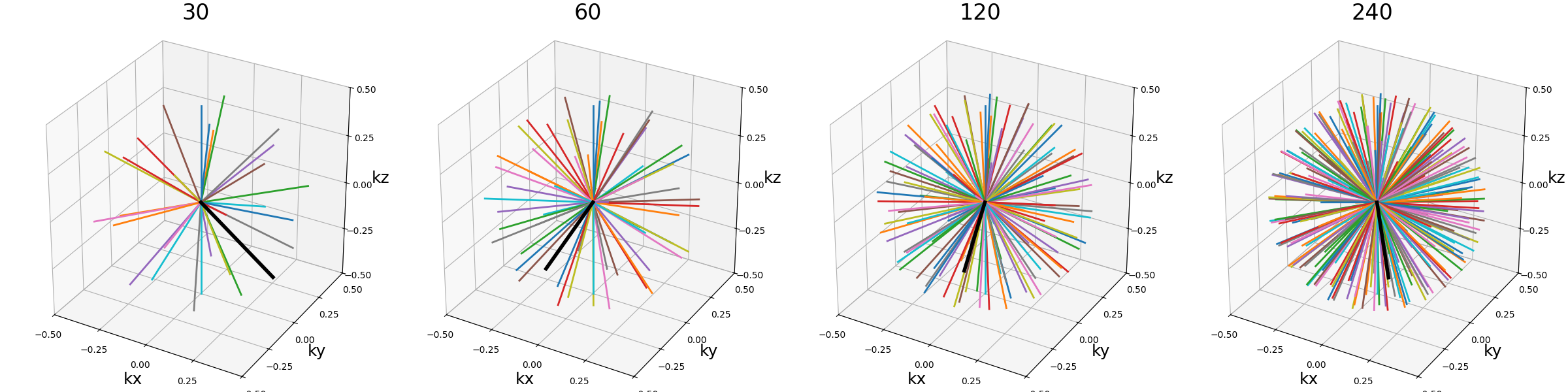
nb_shells (int)

Number of shells, i.e. concentric spheres, used to partition the k-space sphere.

arguments = [1, 2, nb_repetitions // 2, nb_repetitions]
function = lambda x: mn.initialize_3D_helical_shells(
    Nc=x, Ns=Ns, nb_shells=x, spiral_reduction=2
)
show_trajectories(function, arguments, one_shot=False, subfig_size=subfigure_size)

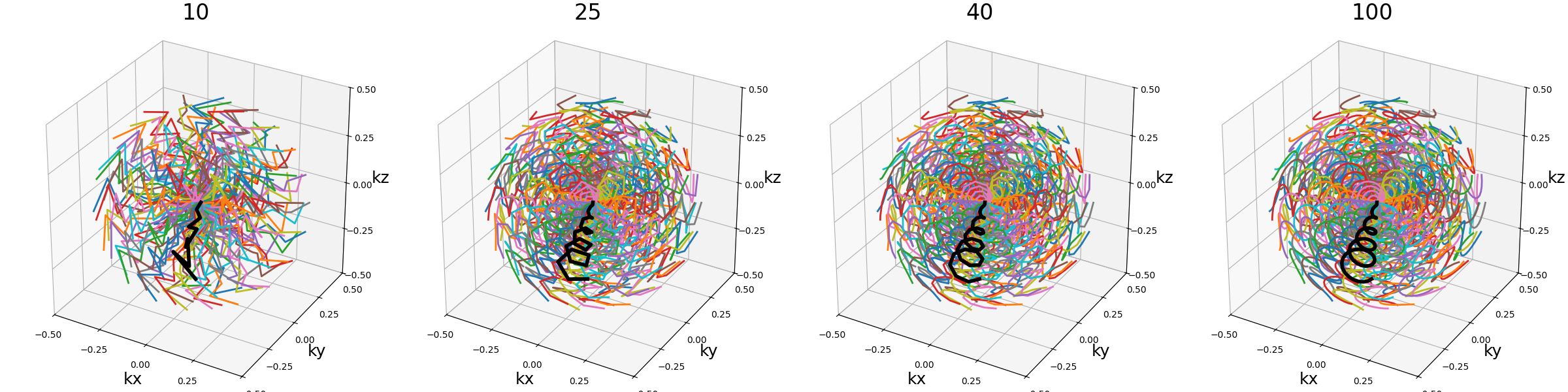
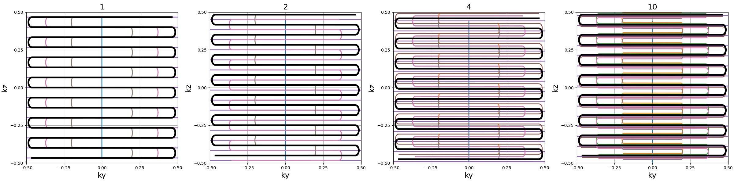
spiral_reduction (float)

Normalized factor controlling the curvature of the spirals over the sphere surfaces. The curvature is determined by Nc and Ns automatically based on [YRB06] in order to provide a coverage with minimal aliasing, but the curve velocities and accelerations might make them incompatible with gradient and slew rate constraints. Therefore we provided spiral_reduction to reduce (or increase) the pre-determined spiral curvature.

arguments = [0.5, 1, 2, 4]
function = lambda x: mn.initialize_3D_helical_shells(
    Nc=Nc, Ns=Ns, nb_shells=nb_repetitions, spiral_reduction=x
)
show_trajectories(function, arguments, one_shot=one_shot, subfig_size=subfigure_size)

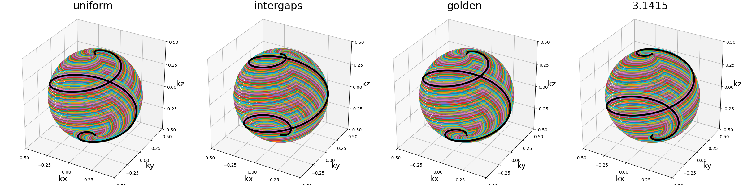
shell_tilt (str, float)

Angle between each consecutive shells (in radians).

arguments = ["uniform", "intergaps", "golden", 3.1415]
function = lambda x: mn.initialize_3D_helical_shells(
    Nc=Nc, Ns=Ns, nb_shells=nb_repetitions, spiral_reduction=2, shell_tilt=x
)
show_trajectories(function, arguments, one_shot=one_shot, subfig_size=subfigure_size)

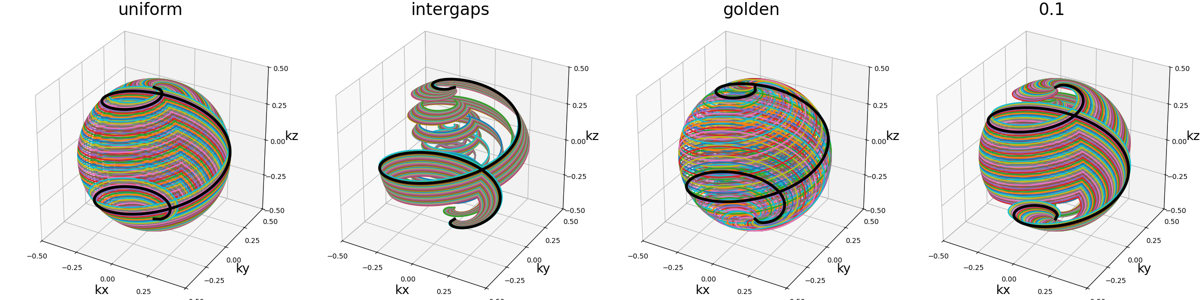
shot_tilt (str, float)

Angle between each consecutive shot over a shell/sphere (in radians). Note that since the number of shots per shell is determined automatically for each individual shell following a density provided in [YRB06], it is advised to use adaptive keywords such as “uniform” rather than hard values.

arguments = ["uniform", "intergaps", "golden", 0.1]
function = lambda x: mn.initialize_3D_helical_shells(
    Nc=Nc, Ns=Ns, nb_shells=nb_repetitions, spiral_reduction=2, shot_tilt=x
)
show_trajectories(function, arguments, one_shot=one_shot, subfig_size=subfigure_size)

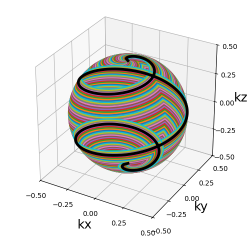
Annular shells

An exclusive trajectory composed of re-arranged rings covering concentric shells with minimal redundancy, based on the work from [HM11]. The rings are cut in halves and recombined in order to provide more homogeneous shot lengths as compared to a spherical stack of rings.

Arguments:

• Nc (int): number of individual shots. See 3D radial

• Ns (int): number of samples per shot. See 3D radial

• nb_shells (int): number of shells used to partition the k-space. It should be lower than or equal to Nc. See helical shells.

• shell_tilt (str, float): angle between each consecutive shell (in radians). (default pi). See helical shells.

• ring_tilt (str, float): angle used to rotate the half-sphere of rings (in radians). (default pi / 2)

trajectory = mn.initialize_3D_annular_shells(Nc, Ns, nb_shells=nb_repetitions)
show_trajectory(trajectory, figure_size=figure_size, one_shot=one_shot)

ring_tilt (float)

Angle (in radians) defining the rotation between the two halves of each spheres, and therefore also the rings recombination. A zero angle, as seen on the first example, results in a simple stack-of-rings, while an angle of \(\pi / 2\) on the third example makes the ring take a right angle.

Note that the angle is discretized over each sphere depending on the number of rings, and therefore the angle might be inaccurate over smaller shells.

An angle of \(\pi / 2\) allows reaching the best shot length homogeneity, and it partitions the spheres into several connex curves composed of exactly two shots.

arguments = [0, np.pi / 4, np.pi / 2, 3 * np.pi / 4]
function = lambda x: mn.initialize_3D_annular_shells(
    Nc, Ns, nb_shells=nb_repetitions, ring_tilt=x
)
show_trajectories(function, arguments, one_shot=one_shot, subfig_size=subfigure_size)

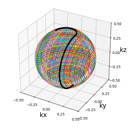
Seiffert shells

An exclusive trajectory composed of re-arranged Seiffert spirals covering concentric shells. All curves have a constant speed and angular velocity, depending on the size of the sphere they belong to.

This implementation is inspired by the propositions from [YRB06] and [SMR18], and also based on works from [Er00] and [Br09].

Arguments:

• Nc (int): number of individual shots. See 3D radial

• Ns (int): number of samples per shot. See 3D radial

• curve_index (float): Index controlling curvature from 0 (flat) to 1 (curvy). (default 0.3). See Seiffert spirals

• nb_revolutions (float): number of revolutions or elliptic periods. (default 1). See Seiffert spirals

• shell_tilt (str, float): angle between each consecutive shell (in radians). (default "intergaps"). See helical shells

• shot_tilt (str, float): angle between each consecutive shot over a sphere (in radians). (default "uniform"). See helical shells

trajectory = mn.initialize_3D_seiffert_shells(Nc, Ns, nb_shells=nb_repetitions)
show_trajectory(trajectory, figure_size=figure_size, one_shot=one_shot)

fMRI trajectories

In this section are presented long trajectories designed for functional MRI to cover the k-space in a few shots, often composed of multiple readouts.

TURBINE

The TURBINE (Trajectory Using Radially Batched Internal Navigator Echoes) trajectory as proposed in [MGM10]. It consists of EPI-like multi-echo planes rotated around any axis (here \(k_z\)-axis) in a radial fashion.

Note that our implementation also proposes to segment the planes into several shots instead of just one, and includes the proposition from [GMC22] to also accelerate within the blades by skipping lines but while alternating them between blades.

Arguments:

• Nc (int): number of individual shots. See 3D radial

• Ns_readouts (int): number of samples per readout. See 3D radial

• Ns_transitions (int): number of samples per transition between two readouts.

• nb_blades (int): number of blades used to group readouts into and partition the k-space. It should be lower than Nc and divide it.

• blade_tilt (str, float): angle between each consecutive blades over the \(k_z\)-axis (in radians). (default "uniform")

• nb_trains (int): number of resulting shots, or readout trains, such that each of them will be composed of \(n\) readouts with Nc = n * nb_trains. If "auto" then nb_trains is set to nb_blades.

• skip_factor (int): factor defining the way different blades alternate to skip lines, forming groups of skip_factor non-redundant blades. (default 1)

• in_out (bool): define whether the shots should travel toward the center then outside (in-out) or not (center-out). (default True). See 3D radial

nb_blades = Nc // 15
trajectory = mn.initialize_3D_turbine(
    Nc, Ns_readouts=Ns, Ns_transitions=Ns // 10, nb_blades=nb_blades
)
show_trajectory(trajectory, figure_size=figure_size, one_shot=one_shot)

Ns_transitions (int)

Number of samples per transition between two readouts. Smoother transitions are achieved with more points, but it means longer waiting times between readouts if they are split during acquisition.

arguments = [1, 50, 100, 200]
function = lambda x: mn.initialize_3D_turbine(
    Nc=Nc,
    Ns_readouts=Ns,
    Ns_transitions=x,
    nb_blades=nb_blades,
)
show_trajectories(function, arguments, one_shot=one_shot, subfig_size=subfigure_size)

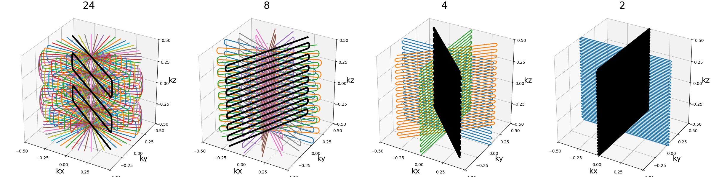
nb_blades (int)

Number of blades used to group readouts into and partition the k-space. More blades means fewer lines per blade. It should be lower than Nc and divide it.

arguments = [Nc // 5, Nc // 15, Nc // 30, Nc // 60]
function = lambda x: mn.initialize_3D_turbine(
    Nc=Nc,
    Ns_readouts=Ns,
    Ns_transitions=Ns // 10,
    nb_blades=x,
)
show_trajectories(function, arguments, one_shot=one_shot, subfig_size=subfigure_size)

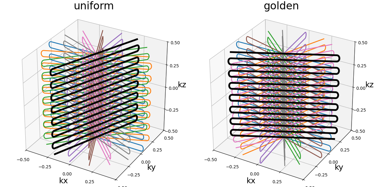
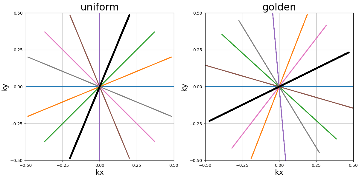
blade_tilt (str, float)

Angle between each consecutive blades over the \(k_z\)-axis (in radians)

arguments = ["uniform", "golden"]
function = lambda x: mn.initialize_3D_turbine(
    Nc=Nc,
    Ns_readouts=Ns,
    Ns_transitions=Ns // 10,
    nb_blades=nb_blades,
    blade_tilt=x,
)
show_trajectories(function, arguments, one_shot=one_shot, subfig_size=subfigure_size)

show_trajectories(
    function, arguments, one_shot=one_shot, subfig_size=subfigure_size, dim="2D"
)

nb_trains (int)

Number of resulting shots, or readout trains, such that each of them will be composed of \(n\) readouts with Nc = n * nb_trains. If "auto" then nb_trains is set to nb_blades.

arguments = [nb_blades, 3 * nb_blades, 5 * nb_blades, 15 * nb_blades]
function = lambda x: mn.initialize_3D_turbine(
    Nc=Nc,
    Ns_readouts=Ns,
    Ns_transitions=Ns // 10,
    nb_blades=nb_blades,
    nb_trains=x,
)
show_trajectories(function, arguments, one_shot=one_shot, subfig_size=subfigure_size)

skip_factor (int)

Factor defining the way different blades alternate to skip lines, forming groups of skip_factor non-redundant blades.

This enables the in-plane acceleration proposed by [GMC22] by increasing skip_factor and nb_blades together by a same factor. Note that using skip_factor superior to nb_blades as below results in k-space areas being not covered by any blade.

arguments = [1, 2, 4, nb_blades + 2]
function = lambda x: mn.initialize_3D_turbine(
    Nc=Nc,
    Ns_readouts=Ns,
    Ns_transitions=Ns // 10,
    nb_blades=nb_blades,
    skip_factor=x,
)
show_trajectories(function, arguments, one_shot=one_shot, subfig_size=subfigure_size)

show_trajectories(
    function,
    arguments,
    one_shot=one_shot,
    subfig_size=subfigure_size,
    dim="2D",
    axes=(1, 2),
)

REPI

The REPI (Radial Echo Planar Imaging) trajectory proposed in [RMS22] and officially inspired from TURBINE proposed in [MGM10]. It consists of multi-echo stacks of lines or spirals rotated around any axis (here \(k_z\)-axis) in a radial fashion, but each stack is also slightly shifted along the rotation axis in order to be entangled with the others without redundancy. This feature is similar to choosing skip_factor equal to nb_blades in TURBINE.

Note that our implementation also proposes to segment the planes/stacks into several shots, instead of just one. Spirals can also be customized beyond the classic Archimedean spiral.

Arguments:

• Nc (int): number of individual shots. See 3D radial

• Ns_readouts (int): number of samples per readout. See 3D radial

• Ns_transitions (int): number of samples per transition between two readouts. See TURBINE

• nb_blades (int): number of blades used to group readouts into and partition the k-space. It should be lower than Nc and divide it. See TURBINE

• nb_blade_revolutions (float): number of revolutions over lines/spirals within a blade over the \(k_z\) axis. See TURBINE

• blade_tilt (str, float): angle between each consecutive blades over the \(k_z\)-axis (in radians). (default "uniform"). See TURBINE

• nb_trains (int): number of resulting shots, or readout trains, such that each of them will be composed of \(n\) readouts with Nc = n * nb_trains. If "auto" then nb_trains is set to nb_blades. See TURBINE

• nb_spiral_revolutions (float): number of revolutions performed from the center. (default 1). See 2D spiral

• spiral (str, float): type of spiral defined through the general archimedean equation. (default "archimedes"). See 2D spiral

• in_out (bool): define whether the shots should travel toward the center then outside (in-out) or not (center-out). (default True). See 3D radial

trajectory = mn.initialize_3D_repi(
    Nc,
    Ns_readouts=Ns,
    Ns_transitions=Ns // 10,
    nb_blades=nb_blades,
    nb_blade_revolutions=nb_revolutions,
    nb_spiral_revolutions=nb_revolutions,
)
show_trajectory(trajectory, figure_size=figure_size, one_shot=one_shot)

nb_blade_revolutions (float)

Number of revolutions over lines/spirals within a blade over the \(k_z\) axis.

Note that increasing it also tends to increase the distance between consecutive lines/spirals, requiring higher gradients and slew rates.

arguments = [0, 0.5, 1, 2]
function = lambda x: mn.initialize_3D_repi(
    Nc=Nc,
    Ns_readouts=Ns,
    Ns_transitions=Ns // 10,
    nb_blades=nb_blades,
    nb_blade_revolutions=x,
    nb_spiral_revolutions=0,
)
show_trajectories(function, arguments, one_shot=one_shot, subfig_size=subfigure_size)

Same but with a spiral pattern instead of radial.

arguments = [0, 0.5, 1, 2]
function = lambda x: mn.initialize_3D_repi(
    Nc=Nc,
    Ns_readouts=Ns,
    Ns_transitions=Ns // 10,
    nb_blades=nb_blades,
    nb_blade_revolutions=x,
    nb_spiral_revolutions=nb_revolutions,
)
show_trajectories(function, arguments, one_shot=one_shot, subfig_size=subfigure_size)

References

[WR94] (1,2)

Wong, Sam TS, and Mark S. Roos. “A strategy for sampling on a sphere applied to 3D selective RF pulse design.” Magnetic Resonance in Medicine 32, no. 6 (1994): 778-784.

[IN95] (1,2)

Irarrazabal, Pablo, and Dwight G. Nishimura. “Fast three dimensional magnetic resonance imaging.” Magnetic Resonance in Medicine 33, no. 5 (1995): 656-662.

[Er00] (1,2)

Erdös, Paul. “Spiraling the earth with C. G. J. Jacobi.” American Journal of Physics 68, no. 10 (2000): 888-895.

[YRB06] (1,2,3,4)

Shu, Yunhong, Stephen J. Riederer, and Matt A. Bernstein. “Three‐dimensional MRI with an undersampled spherical shells trajectory.” Magnetic Resonance in Medicine 56, no. 3 (2006): 553-562.

[Br09] (1,2)

Brizard, Alain J. “A primer on elliptic functions with applications in classical mechanics.” European journal of physics 30, no. 4 (2009): 729.

[Cha+09]

Chan, Rachel W., Elizabeth A. Ramsay, Charles H. Cunningham, and Donald B. Plewes. “Temporal stability of adaptive 3D radial MRI using multidimensional golden means.” Magnetic Resonance in Medicine 61, no. 2 (2009): 354-363.

[MGM10] (1,2)

McNab, Jennifer A., Daniel Gallichan, and Karla L. Miller. “3D steady‐state diffusion‐weighted imaging with trajectory using radially batched internal navigator echoes (TURBINE).” Magnetic Resonance in Medicine 63, no. 1 (2010): 235-242.

[HM11]

Gerlach, Henryk, and Heiko von der Mosel. “On sphere-filling ropes.” The American Mathematical Monthly 118, no. 10 (2011): 863-876

[Pic+11]

Piccini, Davide, Arne Littmann, Sonia Nielles‐Vallespin, and Michael O. Zenge. “Spiral phyllotaxis: the natural way to construct a 3D radial trajectory in MRI.” Magnetic resonance in medicine 66, no. 4 (2011): 1049-1056.

[Pip+11] (1,2)

Pipe, James G., Nicholas R. Zwart, Eric A. Aboussouan, Ryan K. Robison, Ajit Devaraj, and Kenneth O. Johnson. “A new design and rationale for 3D orthogonally oversampled k‐space trajectories.” Magnetic resonance in medicine 66, no. 5 (2011): 1303-1311.

[Bil+15]

Bilgic, Berkin, Borjan A. Gagoski, Stephen F. Cauley, Audrey P. Fan, Jonathan R. Polimeni, P. Ellen Grant, Lawrence L. Wald, and Kawin Setsompop. “Wave‐CAIPI for highly accelerated 3D imaging.” Magnetic resonance in medicine 73, no. 6 (2015): 2152-2162.

[Par+16]

Park, Jinil, Taehoon Shin, Soon Ho Yoon, Jin Mo Goo, and Jang‐Yeon Park. “A radial sampling strategy for uniform k‐space coverage with retrospective respiratory gating in 3D ultrashort‐echo‐time lung imaging.” NMR in Biomedicine 29, no. 5 (2016): 576-587.

[SMR18] (1,2,3)

Speidel, Tobias, Patrick Metze, and Volker Rasche. “Efficient 3D Low-Discrepancy k-Space Sampling Using Highly Adaptable Seiffert Spirals.” IEEE Transactions on Medical Imaging 38, no. 8 (2018): 1833-1840.

[SB21]

Stobbe, Robert W., and Christian Beaulieu. “Three‐dimensional Yarnball k‐space acquisition for accelerated MRI.” Magnetic Resonance in Medicine 85, no. 4 (2021): 1840-1854.

[GMC22] (1,2)

Graedel, Nadine N., Karla L. Miller, and Mark Chiew. “Ultrahigh resolution fMRI at 7T using radial‐cartesian TURBINE sampling.” Magnetic Resonance in Medicine 88, no. 5 (2022): 2058-2073.

[RMS22]

Rettenmeier, Christoph A., Danilo Maziero, and V. Andrew Stenger. “Three dimensional radial echo planar imaging for functional MRI.” Magnetic Resonance in Medicine 87, no. 1 (2022): 193-206.